A Simple Randomized Procedure for Extracting Dominant Patterns Related to the SVD
Dominant Patterns in the Data
One way to think about the SVD is as a procedure for extracting “dominant” patterns in the dataset. If X is an n by m matrix representing the dataset with n data points (rows) and m features (columns), then the principal eigenvectors of $X^TX$ represent some “dominant” patterns in the dataset.
The interesting thing about the SVD is that those patterns are discriminative. They usually discrimnate between two classes or clusters. (Aside: Sometimes they discriminate between one class and the whole dataset. That case can be discovered by looing at the distribution of U[i,:].)
Let v[i] be an eigenvector of (the uncentered covariance matrix) $X^TX$. v[i] is a vector with m numbers. Take the positive numbers – those represent one pattern. Take the negative numbers – those represent another pattern.
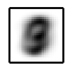
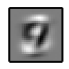
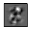
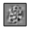
Here is a pattern extracted by the SVD the MNIST dataset containing images of digits:

This pattern represents an image of both a zero and a one.
SVD = Dominant Patterns = Collections of clusters
SVD brings together two views of the data: viewing the dataset as a combination of features, and viewing the dataset as a collection of points.
Let us take the vector v[i] (the eigenvector of the covariance matrix $X^TX$) and compare each data point to v[i] we will find three groups of points:
- those that match the pattern given by the positive numbers
- those that match the pattern given by the negative numbers
- those that fall in between.
The third group will be the largest. This is consequence of the large dimensionality of the data (“the curse of dimenionality”). There could not be a simple rule which splits the data into two meaningful parts for high-dimensional data. (Aside: that’s why linear classifiers do not work well for high-dimensional data)
By the way, matching a data point $i$ to the vector v[j] (note the index $j$) means just executing dot(x[i,:], v[j]). This shall produce the entry u[i,j] in the matrix U from SVD (X = USV’).
The randomized procedure
v1,v2,...,v[k]: sample k = 1024 data points (or some another power 2, the more samples the better)


Step one:
a1 = From the vectors (v1 + v2) or (v1 - v2) choose the one with the larger length
a2 = same for vectors (v3 + v4) and (v3 - v4)
a3 = same for vectors (v5 + v6) and (v5 - v6)
...
a[k/2] = same for vectors (v[k/2 - 1] + v[k/2]) and (v[k/2 - 1] - v[k/2])


Step two:
b1 = choose the longer vector of (a1 + a2) and (a1 - a2)
b2 = same for vectors (a3 + a4) and (a3 - a4)
...

Step three:
Similar to step two, but perform it on b1,b2,...,b[k/4]


There are log(k) steps that return a single vector
...
Implementation
I used scipy to test the procedure on MNIST. The implementation is in the file dominant_patterns.py. The interesting things happen the function combine.
Results
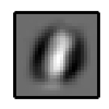
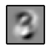
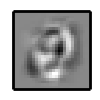
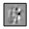
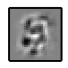
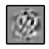
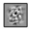
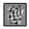
The first four patterns are very similar to what SVD has extracted. Since we do a stage-wise approach the differences between our patterns and the SVD patterns diverge. It is known that even stage-wise SVD via the power method accumulates errors.
|
|
|
|
|
|
|
|
|
|
|
|
|
|

|
|
|
|
|
|
|
|
|
|
|
Interesting futher questions:
- Can you generalize this procedure to produce sparse results (i.e. like sparse SVD, either v[i] or u[i,:] has thresholding, also make it work more like an additive models (with a non-linearity) rather than like a linear model)
- Can you change the objective for optimization (now the objective is to maximize the norm of the final vector) to be more like the objective in Glove (global word vectors)
- verify tha masking effect. That means that removing data points is meaningful. For example if the first principal vector is finding “0” and “1”, then removing “0” and “1”, the procedure is able to discover other patterns not visible before.
- will this procedure work when the data is very sparse? probably not.
- will this procedure work on a summary datastructure, i.e. we extract a summary of the dataset, and then run the greedy optimization on it.
- how is this procedure related to online k-means? Is the divide-and-conquer approach useful for online k-means?
- it also turns out that this procedure is related to so the called reversible-jump MCMC [Wow!]. (check section 3.7 in Introduction to MCMC for Machine Learning” by Michael Jordan et. al. )
An aside on online algorithms
This is an online algorithm. Online algorithms have proven very powerful and useful. For example, online k-means and stochastic gradient descent are the most common members of this family. I should also mention Gibbs sampling and markov chain monte carlo sampling. How do their compare to their batch counterparts? They find better solutions faster (less likely to get stuck in a local optimum) and can consume huge datasets.
Conclusion
Perhaps this procedure is not very useful as something which to work in production. However, I am delighted by the connections it offers to other areas and approaches in Machine Learning. In particular the connection to reversible chain MCMC and online k-means. It is also very exciting that something that simple can discover similar information to the SVD.