Imagine you have a very large collection of documents and you want to organize it (or index it) in such a way so that you can easily
Suffix arrays are one way to go about it. The approach of suffix arrays works by organizing the words in collection in such a way that a linear scan will reveal the number of times an ngram appears in the collection, no matter how long the ngram.
One quite interesting application related to the two questions above is how to extract cheaply all the phrases in a large collection of text.
Suffix arrays are typically explained on a string of text such as “abracadabra”
What we want here is given a substring such as “cadab” to find easily if it is a substring of the original “abracadabra” string. (Instead of array of letters one can consider array of words, the substring in this case is replaced by a phrase containing words.)
So the way we can go about this problem it is to take the original string and create the list of all suffixes:
abracadabra bracadabra racadabra acadabra cadabra adabra dabra abra bra ra a
Then if we search for “cadab” we can see that it will be a prefix of one of the suffixes, namely “cadabra”.
A substring is a prefix of a suffix of the complete string. Therefore, when we search for a substring, we search for a prefix of a suffix. For example, "cadabra" is a suffix, and "cada" is a prefix of length 4 in the suffix "cadabra". If we were searching for "cada", we'd find it to be the prefix of the suffix "cadabra".
One method for speeding up the search is to sort the suffixes and then search with binary search.
When we generate all suffixes of a string of $n$ characters, we need $O(n^2)$ space. This can be avoided if we figure out that we can represent each suffix with a pointer (or offset) in the original string.
Thus, initially the suffixes are represented via the offsets:
0: abracadabra 1: bracadabra 2: racadabra 3: acadabra 4: cadabra 5: adabra 6: dabra 7: abra 8: bra 9: ra 10: a
After sorting we retrieve the suffix string from the offset:
sorted suffixes and the offset in the original string ----------------------------------------------------- start in original array suffix ----------------------------------------------------- 10 "a" 7 "abra" 0 "abracadabra" 3 "acadabra" 5 "adabra" 8 "bra" 1 "bracadabra" 4 "cadabra" 6 "dabra" 9 "ra" 2 "racadabra"
Even though we reduced the memory from the naive $O(n^2)$ to $O(n)$, if we use the obvious sorting method (say plain quick sort), it might take $O(n^2)$ to sort the suffixes. One idea is that we can use a special version of quick sort that works very well for sorting arrays of strings (this version is called multikey ternary quicksort) or let’s just call it fast string sort
Now all that is needed to adapt the implementation(s) from the above article by providing custom implementations for the following functions of strings:
string.length string.charAt(...)
The idea kind of works but a problem appears in a data that contains a lot of duplicate ngrams. For example:
abc abc abc abc
If we attempt to sort and choose the letter ‘b’ as the first pivot we reach the following state:
let extra = abc group 1 (first letter < 'b') abc extra extra extra abc extra extra abc extra abc -------------------- group 2 (first letter == 'b') bc extra extra extra bc extra extra bc extra bc -------------------- group 3 (first letter > 'b') c extra extra extra c extra extra c extra c
Now as one can see, recursing on the first group, since all suffixes there start with ‘a’, we arrive at a group that looks exactly like the second group. Since those groups of suffixes are handled independently, work will be repeated.
A pathological case is data that contains the same character, for example ‘aaaaaaaaaaaaa….aaaa’
The use of the string sorting algorithm is competitive if not many duplicates appear. But no one can guarantee that.
This section is still under construction.
LCP stands for longest common prefix. What LCP means is best explained by an example.
Consider two consecutive suffixes after sorting.
i ind lcp rnk select --------------------------- 0 10 - 0 "a" 1 7 1 1 "abra" 2 0 4 2 "abracadabra" 3 3 1 3 "acadabra" 4 5 1 4 "adabra" 5 8 0 5 "bra" 6 1 3 6 "bracadabra" 7 4 0 7 "cadabra" 8 6 0 8 "dabra" 9 9 0 9 "ra" 10 2 2 10 "racadabra"
For example, in the sorted list, consider the suffix at position $i=6$. This is “bracadabra” Before this suffix, at position $i=5$ we see the suffix “bra”. Since the common prefix of “bra” and “bracadabra” is 3, we write 3 for the LCP of “bracadabra”.
Given the sorted suffixes the LCP array can be computed in linear time. See the implementation in function computeLCP
The LPC array is useful for
Input: 50000 documents Number of total words in those documents: 88 686 630 Size of input array in MBs: 160 (the array is an array of integer ids, each id represents a word)
The time to sort the suffixes is 50 seconds. The same time was achieved by both the fast string sort algorithm and the SA-IS algorithm with implementation by yuta256. However, the fast string sort algorithm may fail to perform well on certain type of data. So the SA-IS algorithm is preferable.
After the suffix array and the LCP (longest common prefix) array are computed it’s a matter of scanning through the LCP array and keeping track of a few counters. This is the function dumpNgrams
The top bigrams are (the scores below are counts):
united kingdom 13463.0 prime minister 13370.0 war ii 12824.0 median income 12762.0 high school 10932.0 university press 10239.0 civil war 9752.0 every females 8878.0 los angeles 8797.0 soviet union 8602.0 per square 8488.0 air force 8413.0 further reading 8190.0 square mile 8184.0 american actor 8110.0 african american 8069.0 press isbn 8027.0
Some interesting trigrams (the scores below are not counts):
dien bien phu -1357.0843587874344 guru granth sahib -1395.1764721438385 tuatha dã© danann -1419.5544827727674 chen shui bian -1431.465076962982 obi wan kenobi -1444.5153566396255 lee kuan yew -1516.8594907003933 chiang ching kuo -1548.9171440014002 gamal abdel nasser -1550.7136811332614 josip broz tito -1579.5224149565151 ursula le guin -1602.9230687266368 ebook kansas cyclopedia -1630.9021398533328 mutant ninja turtles -1645.7369039407974 castilla la mancha -1669.7628172544435 kuala lumpur malaysia -1700.1293484922126 teenage mutant ninja -1719.8348978683298
A working demo is available in the suffix-array project.
]]>query: page_encryption {"page_id":"page_encryption"} {"page_id":"page_clipper"} {"page_id":"page_chip"} {"page_id":"page_key"} {"page_id":"page_keys"} {"page_id":"page_secure"} {"page_id":"page_algorithm"} {"page_id":"page_escrow"} {"page_id":"page_security"} {"page_id":"page_secret"} {"page_id":"page_crypto"}
Please visit the example: Custom Similarity For ElasticSearch
Writing a custom similarity is typically considered a last resort solution although it’s not hard from a developer perspective. The downside typically is (as with any computer code) that you need to test it, profile it, distribute it to the production servers and continue to maintain it as bugs are discovered or the Elasticsearch API changes.
So before choosing this path please make sure that existing similarities and their parameters won’t work. Make sure that extending the similarities with scripting won’t work either. A typical use case for scriptiong is when you want to give a boost to a document based on recency or location. So typically time-based boosting or location boosting is not a good case for a similarity plugin.
However, there could be situations when a custom scoring mechanism is the best option.
A good use case is when you have a well-performing similarity measure (and you are sure of that!), but this similarity is not integrated into Elasticsearch.
One of the simplest recommenation systems that is based on user clicks (or user iteraction with items) is by finding item-to-item correlations. This a type of recommendation system pioneered by Amazon which can be simply described as:
"Most" users who clicked on A also clicked on B.
Even though there are a number of ways to implement such as scoring function, many of those methods require the overlap between the vectors of user clicks for two items.
You have the following situation:
item_a = [user_1, user_50, user_32, user_65, ...] item_b = [user_23, user_50, user_52, user_64, ...]
One simple similarity is the following
clicks_overlap = #distinct users who clciked on both item_a and item_b clicks_a = #distinct users who clicked on item_a clicks_b = #distinct users who clicked on item_b similarity = min(clicks_overlap/clicks_a, clicks_overlap/clicks_b) = clicks_overlap/max(clicks_a, clicks_b)
Another similarity measure popular in the literature on recommendation systems is also based on the aggregate statistics clicks_a, clicks_b, clicks_ab. It is implemented in Mahout. Here is a blog post describing the intuition behind Mahout LLR scoring.
In this blog post I am are going to implement only the first.
One important consideration is that I’m not running on all the click data per user but only on asample. These are not simple random samples, but are aligned. The publication that introduced this method called the sampling method Condional Random Sampling
Elasticsearch can be easily extended with plugins. There are two kinds of plugins: site and jvm. JVM plugins are java code and allow developers to extend the actual engine, while the site plugins are html and javascript. Common use cases for JVM plugins are:
The current use case requires a jvm plugin.
I’ve put a simple project on github that implements the overlap based similarity
Below I’ll describe how such a plugin is developed.
This project is a maven project since it was eaiser to get started. Many of the existing plugins use maven. In principle we can use a gradle or an sbt project.
No matter the build system used, it is important that a file called plugin-descriptor.properties appear in the top level of the built zip or jar file.
unzip overlap-similarity-plugin-0.0.1-SNAPSHOT.jar ls plugin-descriptor.properties
Sample plugin-descriptor.properties
description=Overlap Similarity Plugin version=0.0.1-SNAPSHOT jvm=true name=overlap-similarity-plugin elasticsearch.version=2.1.1 java.version=1.8 classname=stefansavev.esplugins.OverlapSimilarityPlugin
When elasticsearch installs and loads the plugin, it is looking for the plugin-descriptor.properties file.
In my plugin I need to create a class that extends from the Elasticsearch Plugin class
public class OverlapPlugin extends Plugin { @Override public String name() { return "overlap-similarity"; } @Override public String description() { return "Overlap Similarity Plugin"; } public void onModule(final SimilarityModule module) { module.addSimilarity("overlap", OverlapSimilarityProvider.class); } }
In this particular case I’m not implementing modules() or services() functions as I’m not creating any new modules or services. However, I am adding a similarity to the existing SimilarityModule defined in the Elasticsearch codebase. Notice that onModule is not an overriden method and must take as an argument a SimilarityModule type. If we we doing an custom analyzer the signature would be using AnalysisModule instead of SimilarityModule, like so:
//if a custom analyzer was needed public class CustomAnalyzerPlugin extends Plugin{ public void onModule(final AnalysisModule module) { ... } }
The onModule function is called via Reflection and Elasticsearch uses the declaration of the module type (SimilarityModule vs. AnalysisModule) to figure out which object to pass to our plugin.
The custom similarity provider is specified in the custom plugin class (see onModule function). The similarity provider returns a similarity to be used:
package stefansavev.esplugins; import org.apache.lucene.search.similarities.Similarity; import org.elasticsearch.common.inject.Inject; import org.elasticsearch.common.inject.assistedinject.Assisted; import org.elasticsearch.common.settings.Settings; import org.elasticsearch.index.similarity.*; public class OverlapSimilarityProvider extends AbstractSimilarityProvider { private OverlapSimilarity similarity; @Inject public OverlapSimilarityProvider(@Assisted String name, @Assisted Settings settings) { super(name); this.similarity = new OverlapSimilarity(); } @Override public Similarity get() { return similarity; } }
The custom similarity is the most complex of the three classes we have to create. Ignoring the implementation details the custom similarity looks like this:
public class OverlapSimilarity extends Similarity { public float coord(int overlap, int maxOverlap) {...} public float queryNorm(float valueForNormalization) {...} @Override public long computeNorm(FieldInvertState state){...} @Override public Similarity.SimWeight computeWeight(float queryBoost, CollectionStatistics collectionStats, TermStatistics... termStats){...} @Override public Similarity.SimScorer simScorer(SimWeight stats, LeafReaderContext context) throws IOException{...} }
That’s the most complex part of the article, so make sure to take a short break before proceeding.
Suppose our plugin is deployed. First, we need to create a name for our custom similarity
curl -XPUT 'localhost:9200/page_clicks' -d ' { "settings" : { "index" : { "number_of_shards" : 1, "number_of_replicas" : 1, "store": "memory" }, "similarity" : { "custom_similarity" : { "type" : "overlapsimilarity" } } } } '
Second, when we create the mapping we need to specify that we want our custom similarity based on the field. In this particular case I also specify that I want to store only the user_ids (this is “index_options”: “docs”)
curl -XPUT 'localhost:9200/page_clicks/_mapping/pages' -d ' { "properties": { "page_id": { "type": "string", "index": "not_analyzed" }, "user_ids": { "type": "string", "analyzer": "standard", "index_options": "docs", "similarity": "custom_similarity" } } }
We are executing the following queries:
First, we want to get the user_ids for a particular page
curl -XGET 'localhost:9200/page_clicks/pages/_search' -d' { "query" : { "match" : { "page_id" : "page_encryption" } } } '
The result is
"hits":[{"_index":"page_clicks","_type":"page","_id":"AVIyiARRwYU3IsvU-MhY","_score":6.3752785,"_source": { "page_id": "page_encryption", "user_ids": "user_1951 user_3710 user_7497 user_8351 ..." } }]}}
Then we use the returned user_ids to formulate a similarity query with our similarity
curl -XGET 'localhost:9200/page_clicks/word/_search?pretty' -d' { "_source": [ "page" ], size: 20, "query": { "match" : { "user_ids": "user_1951 user_3710 user_7497 user_8351 ..." } }, "aggs": {} } '
I’m running on a dataset based on the 20-newsgroups dataset. I’m imagining each word corresponds to a page (for example in a on online dictionary each word has a page). Each document corresponds to a user_id. I downloaded the 20-newsgroups dataset and prepared the data for elasticsearch with a script.
The prepared data can be added to elasticsearch via the command:
cd example curl -s -XPOST localhost:9200/_bulk?pretty --data-binary "@data.txt"; echo
I’m executing the above two queries in a script and getting the results:
./similar_pages page_algorithm "_source":{"page":"page_algorithm"} "_source":{"page":"page_secret"} "_source":{"page":"page_encryption"} "_source":{"page":"page_clipper"} "_source":{"page":"page_escrow"} "_source":{"page":"page_key"} "_source":{"page":"page_chip"} "_source":{"page":"page_keys"} "_source":{"page":"page_crypto"} "_source":{"page":"page_secure"} "_source":{"page":"page_security"} "_source":{"page":"page_wiretap"} "_source":{"page":"page_nsa"} "_source":{"page":"page_des"} "_source":{"page":"page_encrypted"} "_source":{"page":"page_details"} "_source":{"page":"page_privacy"} "_source":{"page":"page_information"} "_source":{"page":"page_public"} "_source":{"page":"page_independent"}
It makes sense.
When we run a query Elasticsearch (in this particular case) does something like this:
our_similarity = find the similarity based on the field and the specification in the mapping for each user_id (word) in the user_ids field of the query: sim_weight = our_similarity.computeWeight(user_id, global_statistics) #in sim_weight we get access to the so called normalizations or field_length #in our particular case we get access to the total number of clicks per page value_for_query_normalization = sim_weight.getValueForNormalization() query_normalization = 1/sqrt(sum of value_for_query_normalization for all words in the query) for each user_id in the user_ids field of the query: sim_weight = get the similarity weight for the user_id //tell the similarity_weight for each word about the query normalization sim_weight.normalize(query_normalization) total_score_per_page = {} #page_id -> score or document -> score for each user_id (word) in the user_ids field of the query: sim_weight = get the similarity weight for the user_id sim_scorer = our similarity scorer(sim_weight,...) selected_page_ids = get a list of pages which have this user_id (or get a list of candidate documents) for page_id (document) in selected_page_ids: total_score_per_page[page_id] += sim_scorer.score(page_id,...) sort the page_ids in total_score_per_page by their scores and return the top
The above code explains how the SimWeight and SimilarityScorer interact. The key to understanding the Elasticsearch scoring in this particular case is that we need to know the query length (number of user_ids in the query). The query length is given implicitly to the SimWeight class via a call to the normalize method. What we get there is not actually the query length but 1/sqrt(sum of some weights). The weights that are summed in the square root are actually supplied by the SimWeight scorer via getValueForNormalization method - in this case they are 1 for each user_id in the query.
Another statistic we need is the length of the user_ids field. This information is provided to the SimScorer via the simScorer method:
@Override public final SimScorer simScorer(SimWeight stats, LeafReaderContext context) throws IOException { OverlapStats overlapStats = (OverlapStats) stats; //get access to the query length NumericDocValues docNorms = context.reader().getNormValues(overlapStats.field); //get access to field lengths return new OverlapScorer(overlapStats, docNorms); }
Once we have access to the required statistics we can implement the score method in the SimScorer class that will combine them.
The code for Custom Similarity For Elasticsearch is in github with detailed instructions how to run it.
]]>What does it support?
The two most advanced features compared to other databases are search via the inverted index and grouping of the results. It turns out that to build a flexible analytics engine, those two properties are enough.
Let’s say we are building a website like stackoverflow. The main entities are:
The user entity can be represented as:
entity user{ user_id: string first_name: string last_name: string location: string web_site: string about_me: string interests: [string] experience: list[ { role: optional[string] company: optional[string] }] job_search_status: looing|notlooking }
The question entity can be represented as:
entity question{ title: string full_text: string created_at: string last_modified_at: string user_id: string }
entity answer{ full_txt: string created_at: string last_modified_at: string }
curl -XPUT 'localhost:9200/mystackoverflow' -d ' { "settings" : { "index" : { "number_of_shards" : 10, "number_of_replicas" : 1 } } } '
1.1. Verify the index
curl -XGET 'http://localhost:9200/mystackoverflow/'
1.2. Update the index with mappings for a user
curl -XPUT 'localhost:9200/mystackoverflow/_mapping/user' -d ' { "properties": { "first_name": { "type": "string", "analyzer": "standard" }, "last_name": { "type": "string", "analyzer": "standard" }, "location": { "type": "string", "analyzer": "standard" }, "about_me": { "type": "string", "analyzer": "english" }, "interests" : { "type" : "string", "index": "not_analyzed" }, "created_at": { "type": "date", "format": "date_hour_minute_second_millis" } } } '
1.3. Update the index with mappings for a question
1.4 Create the activity log
class ActivityLog{ user_id: string item_type: string (question or answer) item_id: (question or answer) string created_at: date interaction_type: string (create/update (a question or answer), view (a question or answer), upvote, downvote (a question or answer) }
For example, adding a user:
curl -XPUT localhost:9200/mystackoverflow/user/john_smith?pretty -d ' { "first_name" : "John", "last_name" : "Smith", "about" : "I love to go rock climbing", "interests": [ "cplusplus", "go" ] } '
For example, update the about section in a user:
#notice XPOST vs XPUT curl -XPOST localhost:9200/mystackoverflow/user/john_smith/_update?pretty -d ' { "doc": { "about" : "I love to go rock climbing and kayaking" } } '
Update the keywords of a user:
#do not put duplicates in the list curl -XPOST localhost:9200/mystackoverflow/user/john_smith/_update?pretty -d ' { "script" : "ctx._source.interests = (ctx._source.interests + new_item).unique( false )", "params" : { "new_item" : "java" } } '
Number of questions per keyword
curl -XGET 'localhost:9200/mystackoverflow/question/_search?pretty' -d ' { "size": 0, "aggs": { "group_by_tag": { "terms": { "field": "tags" } } } }'
The query has the following behavior:
Since this is a heavy and frequently executed query, it’s best to cache it
curl -XGET 'localhost:9200/mystackoverflow/activity_log/_search??request_cache=true&pretty' -d ' { size: 0, "query": { "filtered": { "query": { "match_all": {} }, "filter": { "range" : { "created_at" : { "gte" : "now-1000d/d", "lt" : "now/d" } } } } }, "aggs": { "group_by_item": { "terms": { "field": "item_id", "size": 2, "order" : { "distinct_users" : "desc" } }, "aggs" : { "distinct_users" : { "cardinality" : { "field" : "user_id" } } } } } }']]>
Clustering is one technique to organize “unstructured” data for the purpose of seeing a “bird’s eye view of the data” It sounds very cool in theory to be able to “just organize” any data in a meaningful way, but in practice there could be short-comings to the clustering approach which people should be aware of. My advice is here to start with the practical or business requirements. Depending on those you should decide if:
From a business perspective if could be best to imagine how people are going to “consume” the results of the clustering, in what user interface will the results be presented. It could be a good idea to manually hand-craft clusters first and then see if the quality is actually achievable by automated methods if there is a need to scale.
This blog post is about some practical techniques to get your clustering to look as good as possible while running as fast as possible.
Are you solving a grouping problem? If so, what intuitive meaning do you want the groups to have? Do you need interpretability or good labels of the clusters?
Are you building a automated taxonomy for the purpose of navigating the data?
Are you in an insight discovery mode where you try to find dominant patterns (or trends)
In practice, I have not seen en many business examples targeted at end end users that expose raw clustering results. Most probably this is because it is hard to guarantee what an end user might see or how the displayed results should be interpreted.
bottom-up clustering (i.e. create clusters by mering points). Preferable when the number of clusters is large (e.g. more than 10000). Small clusters will look good, but big clusters composed hierarchically of small clusters will be bad (not much structure)
top-down clustering (i.e. create clusters by splitting the dataset). Preferable when the number of clusters is small (e.g. 10 to 1000) At the bottom of the hierarchy, points which should have been in the same cluster will end up in multiple clusters. Typically the first level of the hierarchy will look OK.
k-means clustering. Often the choice in practice but good initialization is critical.
density based clustering. Intuitively appealing but it has problems when the points lie in regions with different density.
There are some examples of clustering in two dimensional datasets in scikit-learn website that show that bottom-up hierarchical clustering and DBScan performs the best. DBscan will not perform well when the clusters have different density (this case is typical in practice). Also, as on those datasets, the single link rule will perform extremely well, while in practice it is problematic. The other clustering algorithms seem to fail even those simple datasets.
All clustering problems are going to have big issues with high-dimensional datasets. This is typically the issue in practice: very few points belong “obviously” to a single cluster. It’s very hard to have a few big clusters that capture well the complete dataset when you have multiple dimensions.
One good way to think about clustering is that clustering gives you automatically rules to group the data. Once you have the “rules” clustering is just about apply the rules to your dataset and grouping by those rules. In clustering the grouping criterion is often expressed as a “bag of words and frequencies” if you are clustering text or as a list of numbers, which represent the average over a set of datapoints. Another way to understand the rule is to look at the “closest” data points that fall in the cluster.
Prefer the k-means algorithm unless you need a hierarchy
Decide on the similarity criterion. For text the cosine after tf-idf or Jenson-Shannon divergence are very good choices. The cosine is simpler to understand while the Jenson-Shannon divergence and related similarities will give better performance. To understand which similarity works well one can look at similarity between examples.
Watch for symmetric vs. asymmetric similarities. This means that you have to decide whether to use similarity between examples (this is symmetric) vs. similarity between cluster and example. There are two ways: P(example given cluster) and P(cluster given example)
Remove outliers. For clustering one can define outliers as points which lie is sparse regions of the dataset (i.e. there not many points around them). This can be done efficiently with nearest neighbor search or node centrality in graphs using the SVD.
Decrease dimensionality of the dataset as much as possible.
Use the best initialization possible.
As I said, there are three tips:
decrease the dimensionality of the data (the easiest way is to use the SVD, but there are other good ways)
decrease the size of the dataset
choose “non-outliers” that are farthest apart
The recommended initialization for k-means is the so called farthest-first traversal. It seems to be a standard choice although not many people know about it. Farthest-first traversal means that initial clusters are points that are as far apart as possible. Unfortunately, in many practical situations those points could turn out to be outliers. Removing outliers and/or restricting initial cluster centers to be points in the dense regions is beneficial. Once this is done, farthest-first traversal can be applied 100000 data points from which to select good initial centers. Farthest-first traversal is a quadratic algorithm however using tricks such as a hashing and exploiting the sparsity of a dataset makes this algorithm perform well. If a small number of clusters is needed (for example 100) one can use the SVD and look for clusters centers in the “corners” given by points with largest projections on the singular vectors. The SVD can still be applied successfully even if more cluster centers are needed (e.g. 1000) by applying it multiple times and removing points which are already well fitted by previously selected cluster centers. As a last tip for obtaining good initialization consider the random projection method. This means the following: draw a random line and choose two points with farthest projections on the line. In recent years there are papers on a random initialization called kmeans++. This is a cheap version of farthest first traversal, where points far from the previous points are selected cheaply (or randomly weighted by their distance to previous centers).
Singular Value Decomposition (SVD) is one of the core techniques of large scale data analysis and Data Science. If you have never heard of the SVD, but you know about linear regression, then it’s also worth knowning that SVD is at the heart of Linear Regression. When applied to text SVD is known as Latent Semantic Analysis.
If you want to know or to invest in one big-data tool that should be SVD because with it you can solve (semantic) search, prediction, dominant pattern extraction, clustering and topic modeling. That is why the SVD can be called the Swiss Army Knife of Big Data. I thought this is an original statement but it turns out others have beaten me to make this statement:
Sanjeev Arora: “A Swiss-army knife for provably solving various ‘clustering’ and ‘learning’ problems. (For reference, Sanjeev Arora is one of the top algorithms people today. He is currently a professor at Princeton and is a receiver of the Gödel and Fulkerson prizes.)
Petros Drineas citing Diane O’Leary: “SVD is the Swiss Army knife of linear algebra” (For reference Petros Drineas is one of the top researchers in scalable linear algebra.)
The SVD is one of the few techniques that scale really well. When I say scale I imagine something very concrete. I can convert Wikipedia to the so called latent semantic representation for about 30-60 minutes on a laptop computer with limited memory of 2-4GB. It depends how many passes one wants to do, but the whole process can be done in just three passes. However, if one wants more accuracy one can add more passes. For reference, just looping over the cleaned text of wikipedia while reading the data from disk takes about 5 minutes. The size of the Wikipedia text without formatting is 11GB. Another point of reference is that a more advanced software called Word2Vec (Google Word Vectors) is practically infeasbile with small resources (In my experience Word2Vec will crunch Wikipedia for a week; recently I heard the gensim implementation in Python is a lot faster).
Because of its scalability, output quality and wide applicability, the SVD is there to stay even though the technique dates back to the late 1800. The application of SVD to text, called Latent Semantic Analysis, is now 25 years old. The history of SVD is related to big names in mathematics and statistics like Jacobi, Beltrami, Jordan and Pearson.
Amazingly, the SVD connects core concepts in philosophy, language, mathematics, statistics, natural language processing, information retrieval and algorithms. In mathematics itself SVD is used in geometry, linear algebra and optimization. At the heart of SVD lies deep geometrical intuion, and it is no surprise SVD originated in geometry and not in algebra.
Nowadays, SVD can be employed to make money in e-commerce (recommendation systems), (semantic) search and web advertising. For example, Spotify uses SVD for music recommendations.
One curious trivia piece is that the original paper that proposed to use SVD for text search is called “A Solution to Plato’s Problem: The Latent Semantic Analysis Theory of Acquisition, Induction and Representation of Knowledge”. So there you go establishing a connection to 400 B.C. when Plato and Socrates were debating the nature of knowledge. But ok, what is the connection to the SVD?
Plato’s problem can be stated as “How do people connect the dots (or make inferences from limited knowledge)”? In the words of Chomsky who named this the “Plato’s problem” how is it that through limited experience or exposure to language people acquire advanced concepts they were never taught explicitly.
For example, through the use of SVD a computer can aquire lists containing country names or a list containing vegetable names.
query: germany germany 1.0 italy 0.90 russia 0.89 sweden 0.88 spain 0.87 kingdom 0.87 france 0.86 republic 0.86 netherlands 0.86 poland 0.85 |
query: bulgaria bulgaria 1.0 romania 0.91 croatia 0.89 hungary 0.88 slovakia 0.88 slovenia 0.87 serbia 0.87 macedonia 0.85 ukraine 0.84 albania 0.83 |
query: pepper pepper 1.0 garlic 0.98 sauce 0.98 spices 0.97 onion 0.97 onions 0.97 fried 0.97 boiled 0.97 tomato 0.97 soup 0.97 |
Application of SVD may connect points such as “bulgaria” and “romania” that are two degrees of separation since there are many ways to reach any one from the other one. Connecting points two (or more) degrees of separation allows hidden connection to surface out. |
Follow Me to learn the tricks on how to compute the SVD on Wikipedia in 30 minutes (with approximations). Along the way, you’ll see other fascinating tricks related to scalable methods for high dimensional data. The methods have fancy names like random projections, hashing and sketching. There are also some simple but quite important tricks related to transforming word counts and modeling walks on graphs with matrix multiplication. I also explore the relationship between sparse co-occurence models and dense factorization models (when one is superior to the other - well they are complementary).
Finds a 2-approx to mimimization of maximum intercluster distance (or maximum cluster radius). The algorithm is efficient O(k*n) for k clusters. The points need to satisfy the triangle inequality to match the approx. factor.
Algorithm: Initially all points are in the same cluster with one arbitrary point denoted as the “head” of the cluster.
Iteration 1: Step 1: From the first cluster (which contains all points) choose the point furthest from the head. Step 2: Go over the points in the first cluster and partition them into two: we move a point to the second (just created cluster) if the distance to the head of the second cluster is smaller than to the distance to the head of the first cluster.
Iteration 2: Now we have two clusters. From the first cluster find the furthest point from the head of the cluster; From the second cluster find the furthest point from the head of the second cluster. Choose the point furthest from its respective “head”. Put that point in a third cluster. Go over the points in the first and second clusters and move those of them that are closer to the head of the first cluster than their respective “heads”
and so on until k clusters have been created.
If the data is sparse the distances may not be very reliable. Use the SVD. For initialization of the first two clusters one can also use the SVD (the two furthest points along the first principle direction) If a small number of clusters is required (e.g. k = log(n)) this algorithm will do. For each point we maintain the distance to the current head. When a new head is created we need to evaluate the distances from the new head to each of the points. May be one can use some approximation since we need to know only the points that are closer to the newly opened cluster. One can also do a bottom up pass as a preprocessing step to merge some points which are “obviously” close. In this way n is reduced.
For an alternative description see Figure 4 in Dasgupta: Performance guarantees for hierarchical clustering. http://cseweb.ucsd.edu/~dasgupta/papers/hier-jcss.pdf
Based on the furtest first traversal describes how to create a tree (hierarchy of clusters) with some optimality properties.
The idea is that first firthest first traversal is run so that the points are numbers. 1 is the first point, 2 is the second point added and so on. While doing that, we are actually defining clusterings with k clusters. First k = 1, then k = 2, and so on. As we go to larger values of k, the radiuses of the clusters shrink. We are using the distances between the cluster centers. $R_i$ is the min. distance from cluster center $i$ to the previous cluster centers (1,2,…, i - 1). Now we bucket those radiuses. If $R$ is the radius of the complete dataset, then the buckets are containing points of radiuses:
It’s probably (although not mentioned) that the number of points in the buckets increases by a factor of 2 with each level.
At the next stage of the algorithm we are building a tree. We start with point 1 (“head” of the first cluster containing all the points). We then take the second point, and we have a tree with two nodes. Next we pick point 3. 3 will be added under 1 or 2 – whichever it is closer. Suppose we add it under 2. We have:
/\ / \ 1 2 / / 3
Next we pick 4. It can be potentially added under 1, 2 or 3. However, we also consider the buckets based on the radiuses $R_i$. Suppose that 4 is at bucket (R/4, R/2) and 3 is at the same bucket. We cannot add 4 under 3 because it will not decrease the radius of 3. So we add 4 under 1 or 2 – which is closer - suppose 1. What we want to achieve with this is a guarantee that the radius is halved or even more than halved.
/\ / \ 1 2 / / / / 4 3
link. This is something that is potentially faster and more accurate than LDA.
Stage 1:
The key is first to throw out words from each document if they do not appear above a threshold. The threshold is individually decided for each word. The reason is that some words e.g. “run” belong to a topic (“sports”), but can also be used outside of a topic (“to run an election”). Therefore, we put a threshold above which there is a higher chance that the word “run” is used indicatively of a topic.
Stage 2:
Then we are going to use the “truncated” documents to build topic clusters. We want that the correlations between two “truncated” documents are more “truthful”. We also need a substantial number of documents (those are available in practice) to overcome the “data loss” from the truncation. We cluster those “truncated” documents by first representing them in the SVD space and then using a k-means approximation algorithm (e.g. farthest first traversal on the SVD representation). Then we refine the k-means approximation using the typical k-means iterative scheme. Notice that they run the iterative k-means stage on the truncated matrix, not the SVD’ed one. Each cluster defines a topic vector. We also keep the individual documents in the topic.
Stage 3:
Clean up the topics via catchwords. The idea is that only a few words are enough to indicate a topic – so called catch words. The other words are adding more noise than signal. Given that we already have the topics, the catch words are going to stick out: be more frequent – they take some of the highest entries.
Notes: instead of thresholds, one can consider a hypothesis test: “is that word coming from the distrubtion of a document (or topic) or is coming from a general background distribution”. It could be more reliable that some thresholds which are picked to make the proofs work.
One way to think about the SVD is as a procedure for extracting “dominant” patterns in the dataset. If X is an n by m matrix representing the dataset with n data points (rows) and m features (columns), then the principal eigenvectors of $X^TX$ represent some “dominant” patterns in the dataset.
The interesting thing about the SVD is that those patterns are discriminative. They usually discrimnate between two classes or clusters. (Aside: Sometimes they discriminate between one class and the whole dataset. That case can be discovered by looing at the distribution of U[i,:].)
Let v[i] be an eigenvector of (the uncentered covariance matrix) $X^TX$. v[i] is a vector with m numbers. Take the positive numbers – those represent one pattern. Take the negative numbers – those represent another pattern.
Here is a pattern extracted by the SVD the MNIST dataset containing images of digits:
This pattern represents an image of both a zero and a one.
SVD brings together two views of the data: viewing the dataset as a combination of features, and viewing the dataset as a collection of points.
Let us take the vector v[i] (the eigenvector of the covariance matrix $X^TX$) and compare each data point to v[i] we will find three groups of points:
The third group will be the largest. This is consequence of the large dimensionality of the data (“the curse of dimenionality”). There could not be a simple rule which splits the data into two meaningful parts for high-dimensional data. (Aside: that’s why linear classifiers do not work well for high-dimensional data)
By the way, matching a data point $i$ to the vector v[j] (note the index $j$) means just executing dot(x[i,:], v[j]). This shall produce the entry u[i,j] in the matrix U from SVD (X = USV’).
v1,v2,...,v[k]: sample k = 1024 data points (or some another power 2, the more samples the better) Step one: a1 = From the vectors (v1 + v2) or (v1 - v2) choose the one with the larger length a2 = same for vectors (v3 + v4) and (v3 - v4) a3 = same for vectors (v5 + v6) and (v5 - v6) ... a[k/2] = same for vectors (v[k/2 - 1] + v[k/2]) and (v[k/2 - 1] - v[k/2]) Step two: b1 = choose the longer vector of (a1 + a2) and (a1 - a2) b2 = same for vectors (a3 + a4) and (a3 - a4) ... Step three: Similar to step two, but perform it on b1,b2,...,b[k/4] There are log(k) steps that return a single vector ...
I used scipy to test the procedure on MNIST. The implementation is in the file dominant_patterns.py. The interesting things happen the function combine.
The first four patterns are very similar to what SVD has extracted. Since we do a stage-wise approach the differences between our patterns and the SVD patterns diverge. It is known that even stage-wise SVD via the power method accumulates errors.
This is an online algorithm. Online algorithms have proven very powerful and useful. For example, online k-means and stochastic gradient descent are the most common members of this family. I should also mention Gibbs sampling and markov chain monte carlo sampling. How do their compare to their batch counterparts? They find better solutions faster (less likely to get stuck in a local optimum) and can consume huge datasets.
Perhaps this procedure is not very useful as something which to work in production. However, I am delighted by the connections it offers to other areas and approaches in Machine Learning. In particular the connection to reversible chain MCMC and online k-means. It is also very exciting that something that simple can discover similar information to the SVD.
]]>X = U*S*Vt X is n by m Vt is k by m
On can think of the vectors Vt[i,:] (to use the Python notation) as patterns. Then the SVD is computing those patterns (the matrix Vt) as well as the overlap of points of the dataset (X[i,:]) with the patterns. The coefficients of the overlap (overlap is just a dot product) are available in the vector U[i,:].
For the purposes of this demo, I ran SVD on the MNIST dataset. The MNIST dataset contains images of digits. Below are some of the patterns that SVD extracted. Given the data in MNIST it is not surprising that the first few “patterns” resemble digits.
It takes a bit of experience with the MNIST data to interpret the patterns correctly. You can think that the first pattern is 9. However, this is simply the average of all images in the dataset. It turns out that if you average all images of digits of 0 to 9 in MNIST, what you get looks like a 9 (or a 0). The second image which looks like 0 is actually SIMULTANEOUSLY both a 0 and 1. “0” is represented by the red pixels while “1” is represented by the yellow-white pixels. The next two plots look like 3 (yellow) interleaved with 9(red) and 3 (yellow) interleaved with 0(red).
This brings us to the one property of the SVD, namely that the patterns or the vectors Vt[i,:] contain both positive and negative values. The positive values may represent one pattern while the negative can represent another pattern (see above: in the same Vt[i,:] we see simultaneously both a “0” and a “1”).
This property may or may not be desirable. If you want to have “clean patterns” the SVD is not the best technique. Some people will prefer the so called non-negative matrix factorization methods which will restrict the patterns to have only positive values. However, even if you attempt a non-negative matrix factorization, it’s very likely that the aglorithm you use is making use the SVD to find a good starting condition from which to extract the patterns. So the SVD is useful, just needs a refinement.
Looking at patterns Vt[i,:] for high values of i, we actually stop seeing patterns that resemble the original inputs. Maybe one pattern is the union of “3” and a “4”. Then anoth
Nevertheless, those patterns are still used to represent the original inputs. The original inputs are just the sum of such patterns appropriately weighted.
One way to think of the SVD is as a way to find a more compact representation of the data. In doing so, the SVD follows (what is equavalent) to a very greedy strategy. First, it finds a dominant pattern in the dataset. Then it just subtracts it from each of the points in the dataset. However, at every iteration the same points are used (without being reweighted). At the end, what will be left from the original inputs will have a lot less structure and may start looking like noise.
Here are the patterns extracted for i = 60, 70, 80, 90. There is still some structure left. However, you cannot say that the original images were digits. They could have been letters and by looking at those patterns it will be impossible to know.
If you are hoping to run the SVD on MNIST (or another dataset) and get out “clean” patterns or clean clusters, it will probably not happen. This is not what the SVD does. However, a repeated application of the SVD might be able to extract some dominant patterns that have high overlap with actual data points. Here is (one variation of) the trick:
X: full dataset U,s,Vt = svd(X, k = 50) #apply SVD for the first time take the first left singular vectors (e.g. 10 or 50) remaining_point_ids = range(0, n) for each column i in U: point_ids = sort the values U[:,i] and extract the point ids corresponding to top highest and top lowest remaining_point_ids.remove_all(point_ids) X1 = X[remaining_point_ids,:] #create a new dataset with the remaining point ids again apply SVD, find points with very high/very low U[:,i] and remove them
The following are some “meaningful patterns” extracted in this way (see the code )
0 | ||||||||||
---|---|---|---|---|---|---|---|---|---|---|
1 | ||||||||||
2 | ||||||||||
3 | ||||||||||
4 | ||||||||||
5 | ||||||||||
6 | ||||||||||
7 | ||||||||||
8 | ||||||||||
9 |
(The “0” and “1” look the same, however “0” is the white pixels, while “1” is the black pixels.
The moral is “Don’t give up on the SVD, just apply it a few times.”
There is a publication that applies SVD in a similar fashion:
]]>There are already some good resources on the web (presentations, scikit learn demos and documentation).
Official page scikit-learn page on classification with 20 newgroups
Another tutorial on text classification with Scikit learn, by Jimmy Lai
remove = ('headers', 'footers', 'quotes') #remove headers, signatures to make the problem more realistic categories = None #load all categories data_train = fetch_20newsgroups(subset='train', categories=categories, shuffle=True, random_state=42, remove=remove) data_test = fetch_20newsgroups(subset='test', categories=categories, shuffle=True, random_state=42, remove=remove)
vectorizer = TfidfVectorizer(sublinear_tf=True, smooth_idf = True, max_df=0.5, stop_words='english') X_train = vectorizer.fit_transform(data_train.data) #fit_transform on training data X_test = vectorizer.transform(data_test.data) #just transform on test data
When using a custom text analysis pipeline
def tokenize(text): tokens = nltk.word_tokenize(text) #include more steps if necessary return tokens vectorizer = TfidfVectorizer(tokenizer=tokenize, #provide a tokenizer if you want to sublinear_tf=True, smooth_idf = True, max_df=0.5, stop_words='english')
feature_names = vectorizer.get_feature_names() ch2 = SelectKBest(chi2, k=opts.select_chi2) X_train = ch2.fit_transform(X_train, y_train) X_test = ch2.transform(X_test) selected_feature_names = [feature_names[i] for i in ch2.get_support(indices=True)]
#need (X_train, y_train) and (X_test, y_test) clf = MultinomialNB(alpha=.01) #or clf = LinearSVC(loss='l2', penalty="l2", dual=False, tol=1e-3, C = 10) clf.fit(X_train, y_train) pred = clf.predict(X_test) accuracy = metrics.accuracy_score(y_test, pred)
Run the script https://github.com/stefansavev/demos/blob/master/text-categorization/20ng/20ng.py
python 20ng.py --filtered --all_categories
You’ll see this output. You want to look at the accuracy for different methods. The methods reported here are linear classifiers. All the accuracies are pretty much the same between 0.69 and 0.7. Notice the “–filtered” option. This option removes some of the headers to make the task more realistic. If headers are not removed the accuracy is higher.
11314 documents - 13.782MB (training set) 7532 documents - 8.262MB (test set) 20 categories Using TfidfVectorizer feature extraction on training set (tokenization) in 12.127502s at 1.136MB/s n_samples: 11314, n_features: 101323 feature extraction on test set (tokenization) in 5.820425s at 1.419MB/s n_samples: 7532, n_features: 101323 Results: RidgeClassifier(alpha=1.0, class_weight=None, copy_X=True, fit_intercept=True, max_iter=None, normalize=False, solver='lsqr', tol=0.01) train time: 3.992s test time: 0.105s accuracy: 0.702 dimensionality: 101323 density: 1.000000 LinearSVC(C=1, class_weight=None, dual=False, fit_intercept=True, intercept_scaling=1, loss='l2', multi_class='ovr', penalty='l2', random_state=None, tol=0.001, verbose=0) train time: 6.567s test time: 0.030s accuracy: 0.697 dimensionality: 101323 density: 1.000000 SGDClassifier(alpha=0.0001, class_weight=None, epsilon=0.1, eta0=0.0, fit_intercept=True, l1_ratio=0.15, learning_rate='optimal', loss='hinge', n_iter=50, n_jobs=1, penalty='l2', power_t=0.5, random_state=None, shuffle=False, verbose=0, warm_start=False) train time: 8.887s test time: 0.105s accuracy: 0.701 dimensionality: 101323 density: 0.378897 MultinomialNB(alpha=0.01, class_prior=None, fit_prior=True) train time: 0.225s test time: 0.079s accuracy: 0.696 dimensionality: 101323 density: 1.000000]]>
The following is a common notation
X is an n by m matrix rows = data points columns = features n: number of rows (data points) m: number of columns (features)
This is the following transformation:
Transform the dataset: for each column i of X: column_i = X[:,i] X[:,i] = column_i - mean(column_i) Let U,S,V = svd(X, k = 100) -- svd after transformation U is an n by k orthonormal matrix S is an k by k diagonal matrix V is an m by k orthonormal matrix Then we have a new representation of the dataset. Option a) U (n by k matrix; k new features) Option b) U*diag(S) Option c) V*diag(sqrt(S*S/(S*S + 1.0))) Option d) V*diag(f(S)), f(s) = if s >= threshold 1/s else 0.0
Geometrically PCA corresponds to “centering the dataset”, and then rotating it to align the axis of highest variance with the principle axis.
Since we use the SVD to compute the PCA, the question is really whether it makes sense to center our dataset by subtracting the means.
A related question arises in the context of linear regression: does it make sense to subtract the means from our variables (as well as divide by standard deviation). This is the so called Z-score normalization. One way to answer this question is to say that because those transformations (subtracting and dividing) are linear transformations of the input and because linear regression is also a linear transformation, it does not matter whether normalizations are carried out. This is true for standard linear regression. However, in practice we do L2-penalized regression (also called ridge regression or Bayesian linear regression). Then the transformation actually matters. For the penalized version of regression both sustracting the mean and dividing by standard diviation are likely to be harmful transformations.
Here we’ll just look at the case of subtracting the means. In many problems our features are positive values such as counts of words or pixel itensities. Typically a higher count or a higher pixel itensity means that a feature is more useful for classification/regression. If you subtract the mean then you are forcing features with original value of zero have a negative value which is high in magnitude. This means you just made the features values that are non-important to the problem of classification as important as the most important features values.
The same reasoning holds for PCA. If your features are least sensitive towards the mean of the distribution, then it makes sense to subtract the mean. If the features are most sensitive towards the high values, then subtracting the mean does not make sense.
In some problems such as image classification or text classification (with bag of words models) we can see empirically that the first right singular vector of the SVD is very similar to a vector computed by averaging all data points. In this case, in the very first step of SVD (if you think of SVD as a stage-wise procedure), SVD takes care of global structure. In the case of PCA, PCA takes care of global structure by substracting the means.
Here is one way to think of the first singular component of the SVD:
col_means_vector = [col_mean_1, col_mean_2, ..., col_mean_m] = the means of the features L2-normalize col_means_vector V[:,1] = col_means_vector # col_means_vector plays the role of V[:,1] U[1,1] = X[1, :].dot(V[:,1]) # this plays the role of a correlation; the result is a scalar U[1,2] = X[2, :].dot(V[:,2]) ... normalize U[:,1] X[1,:] = X[1,:] - s1 * U[1,:] * V[:,1].T #remove global structure X[2,:] = X[2,:] - s1 * U[2,:]* V[:, 1].T ...
So, the column means play a role but in a different way than in the PCA procedure.
]]>Thresholded Correlation Matrix more easily computed with SVD
“A Tutorial on Principal Component Analysis”, Jonathon Shlens
Mathematical Facts about SVD (with view to Signal Processing) by S. J. Orfanidis
“Finding structure with randomness: Probabilistic algorithms for constructing approximate matrix decompositions”, Nathan Halko, Per-Gunnar Martinsson, Joel A. Tropp. A nice approach showing how to scale SVD to really large datasets.
Blog on benchmarking sparse vs. dense SVD in scipy (Dense SVD is faster but takes more memory and is not applicable to large sparse matrices)
Computation of the Singular Value Decomposition using Mesh-Connected Processors by Brent, Luk, Loan (an old paper showing a number of algorithms for SVD)
Versatality of Singular Value Decomposition by Ravi Kannan ( backup link)
Topic Modeling: A Provable Spectral Method by Ravi Kannan (Topic Modeling: A Provable Algorithm)
Clustering: Does theory help? by Ravi Kannan (backup link to slides)
Theory and Big Data by Ravi Kannan (how to apply provably fit a mixture of k Gaussians with the SVD)
Low Rank Approximation and Regression in Input Sparsity Time by Kenneth L. Clarkson and David P. Woodruff (Nearly best rank k approx to A can be found in time linear in the number of non-zero entries in A)
Simple and Deterministic Matrix Sketching by Edo Liberty (essentially running an algorithm for online SVD with small memory; very simple to implement but requires computing the SVD on a small matrix a large number of times.)
When the dataset has two features, one can visualize the whole dataset on a 2D plot.
Let the data be represented by the matrix $X$ where rows are data points and columns are features.
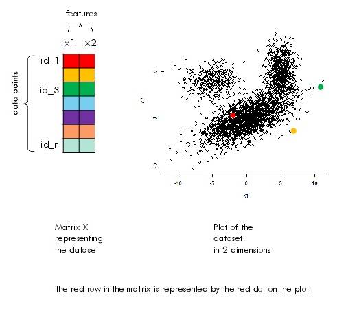
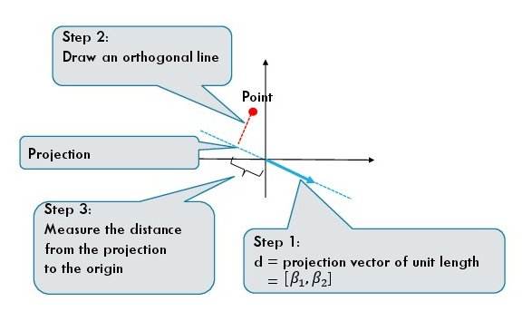
For a one dimensional projection we require a direction which is given by a unit vector $d = [\beta_1, \beta_2]$. The projection of each data point is given by the dot product of the feature vector and the direction:
The above equations give us a procedure to geometrically find the projection of a data point.
The projection of a single point is not informative unless we compare it with the projection of all other points.
Projecting the whole dataset in one dimension gives us a histogram. This histogram is somewhat informative because it may reveal some structure from the original dataset.
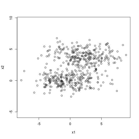
Here is an example. This dataset has two clusters.
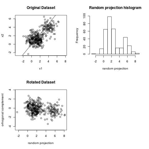
We can observe the clustering structure in the projection above. However, we cannot observe the clustering structure on the projection below.
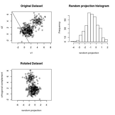
It is known that PCA (a technique related to SVD) is related to finding projections where the histograms are as wide as possible (a wide histogram means large variance). The projection of largest variance is the widest histogram. However, the largest variance projection does not necessarily capture the clustering structure or separability between clusters. This is somewhat of a textbook statement since many textbooks mention this fact.
In the example below we have two clusters which are separable across the axis $x_2$. The dominant right singular vector is however along the direction $x_1$. The singular values are 15 and 6 which tell us that the variance along $x_1$ is about 2.5 times larger than the variance along $x_2$. The clustering structure is revealed however by the second right singular vector of the SVD which is along $x_2$.
It is an interesting question whether for a given dataset we can find one dimensional projections from which you can read the clustering structure (i.e. the histogram of the projection has two peaks and you can guess the clusters from the histogram). This is not possible.
Here is an example with three spheres at equal distance from each other. When projected in one dimension we are never going to see the clusters clearly.
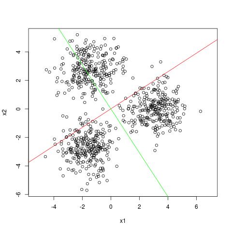
The red and green line are the first and second dominant singular vectors.
However, SVD is still useful for finding clusters in the dataset (see my blog post on SVD and clustering [TO APPEAR]).
Imagine that the data lies on a unit sphere. This is the case when the cosine similarity is used. As it can be seen from the figure below points which are projected in the corners of the projection line are likely to be situated in a much smaller region than points which are projected in the middle. One can have two points projected in the middle which are diametrally opposite each other. In the figure, those are some of the yellow points.
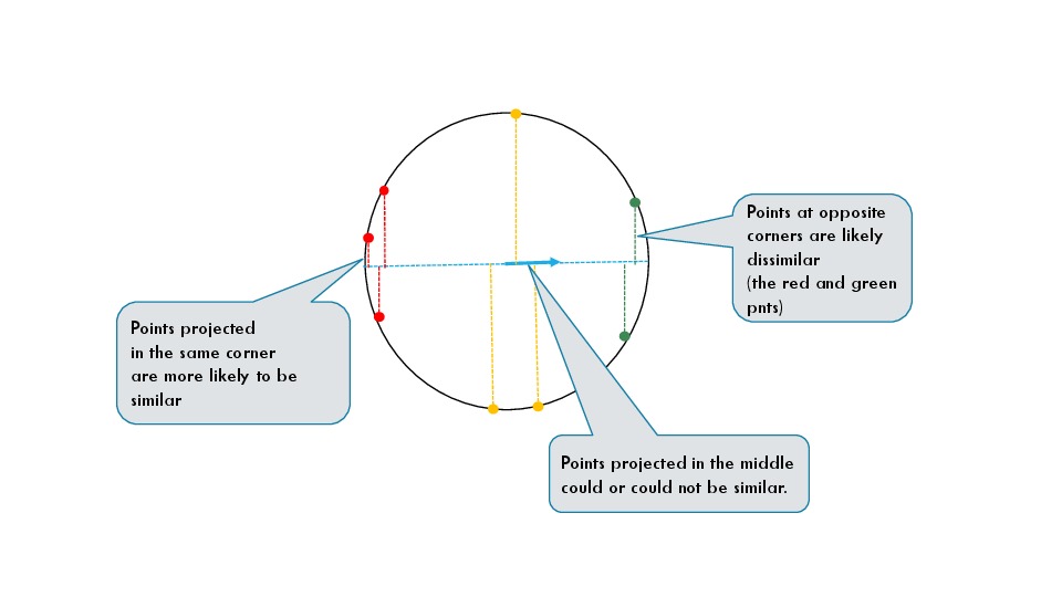
The value of thie statement is that if you take some points projected in one of the corners, those points are likely highly similar. On the other hand, SVD will choose projections for which more data is projected in the corners. This means that the SVD extracts some dominant patterns from the data.
The last statement is used as a heuristic for initialilization of the K-Means clustering algorithm. In the three cluster example above (titled: no one dimensional projection can capture clustering structure), one can see that three of the four corners of the projections contain points from distinct clusters. Points from different corners could be useful for initial centroids in K-means.
Some of the intuition about one dimensional projections carries over to high dimensions. In particular, a one dimensional projection (the histogram) is a view of the dataset also in high dimension. However, it is a much noiser view than a projection in 2D.
In high dimensions it is much more likely that most of the dataset ends up in the middle of the histogram. Why is that? Think of the case of documents on the web. What is a projection is this case? It is two sets of words each representing a topic (why two sets? because the line on which we project has two directions). As an example of two sets of words consider sports and politics. Now projecting a point means that we compare a document on the spectrum from sports and politics. Most documents will be about neither of those things. So those documents (datapoints) are projected close to 0. Projection is dot product and dot product is overlap. A random document will have no overlap with sports or politics. So, in high-dimensions for most possible projections, most of the dataset is projected in the middle. (There is a formal mathematical theorem about this phenomenon.)
The intuition from 2D about the corners of the projections carries over. This means that we should seek interesting structure in the corners. However, there are too many corners in high dimensions and too little data projected on those corners.
The following is the common notation:
The SVD of $X$ is given by
We can write this equation as
This is possible because $V V^T = I$ ($V$ is an orthonormal matrix).
Let us take $V$ to have only one column (this is the truncated SVD with $k = 1$), i.e.$V$ is a single column vector of dimension $m$. This is a projection direction as we described above. Now $U$ is a single column vector $u$ as well, however of dimension $n$. In this case $S$ is a single number $s_1$. $u$ contains the coordinates of the projected points.
We know the following is the best rank-1 approximation to the matrix $X$:
Therefore, we can argue that the projection on the first component of the SVD is the projection that will in some sense “best preserve” the dataset in one dimension. Typically this first projection of the SVD will capture “global structure”.
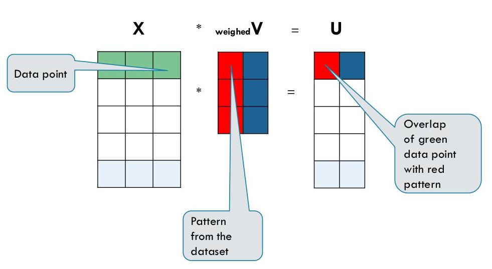
One way heuristic way to think about the first component is as follows. Think of $v_i$ as the average of the $i$-th column; think of $u_j$ as the average of the $j$-th row. This procedure is (sometimes) a heuristic approximation to the SVD with one dominant component when the dataset has global structure. You can see that this is confirmed in the MNIST dataset example below.
One way to define “interesting” is away from normal. One way to be away from normal is to have high variance (heavier tails). The PCA takes exactly this route. It finds the projections which have the highest variance. One critical difference from the SVD is that PCA is SVD on the data after subtracting the means.
Here we want to see how the projections that the SVD produces look like. The MNIST dataset consists of 42000 images. Each image is represented as a 784 dimensional vector. One can obtain this digit recognizer dataset from Kaggle.
I use the following code to read the data and compute the matrix V
train_data <- read.csv('../data/train.flann', header = FALSE, sep = " ") X <- sqrt(data.matrix(train_data)) num_examples <- dim(X)[1] #n num_features <- dim(X)[2] #m #The sample covariance matrix XtX <- (t(X) %*% X)/(num_examples - 1) s <- svd(XtX)
The projections are computed with the following code:
k = 100 #number of singular vectors wanted V = s$v[, 1:k] lam <- 50 d <- s$d[1:k] weights <- sqrt(d/(d + lam)) Vweighted <- s$v[, 1:k] %*% diag(weights) projections = X %*% Vweighted
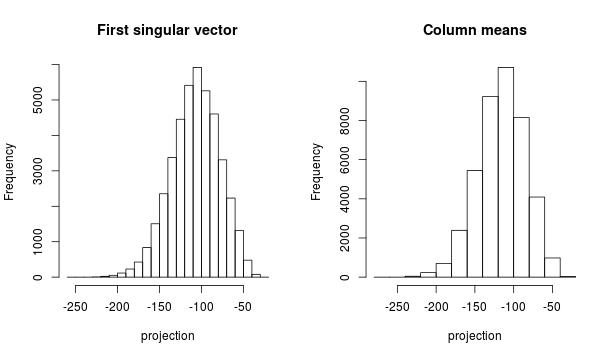
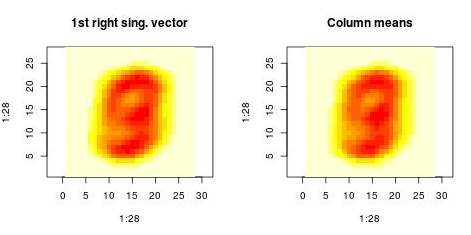
First, I want to make sense of the first projection. We compare the projection on the first right singular vector (on left plot) and the projection on the centroid of the dataset (right plot). Those histograms are very similar and the correlation coefficient beween both projectons is 0.999
This is the code I used to compute the histograms above.
X_colMeans = -colMeans(X) #projection on the column means proj_colMeans = X %*% matrix(X_colMeans, byrow = FALSE) hist(projections[,1], xlab = "projection", main = "First singular vector") #divistion by norm of col means to put the data on the same scale as projections[,1] norm_colMeans = sqrt(sum(X_colMeans * X_colMeans)) #107.6 hist(proj_colMeans/norm_colMeans, xlab = "projection", main = "Column means") cor(projections[,1], proj_colMeans)
This means that the SVD first finds the global structure by “averaging” all images. Then it subtracts this structure and contininues recursively to find additional structure.
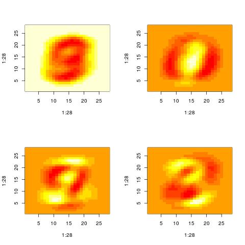
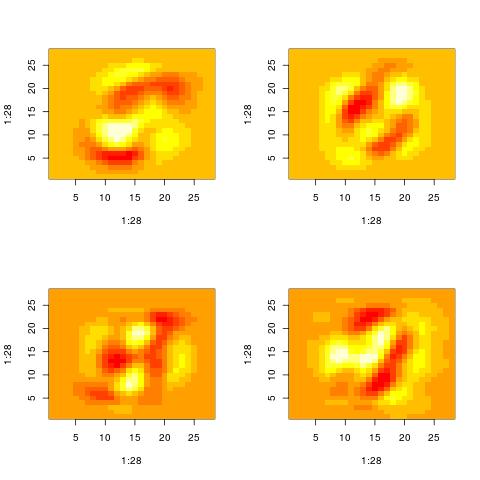
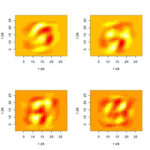
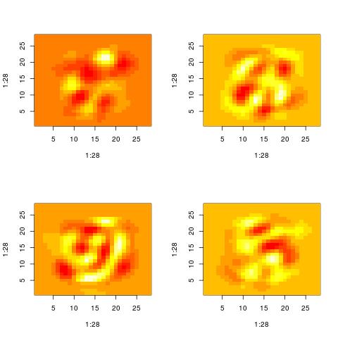
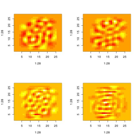
We can also examine the “patterns” present in the right singular vector ($v_1$) and in the vector constructed by averaging columns:
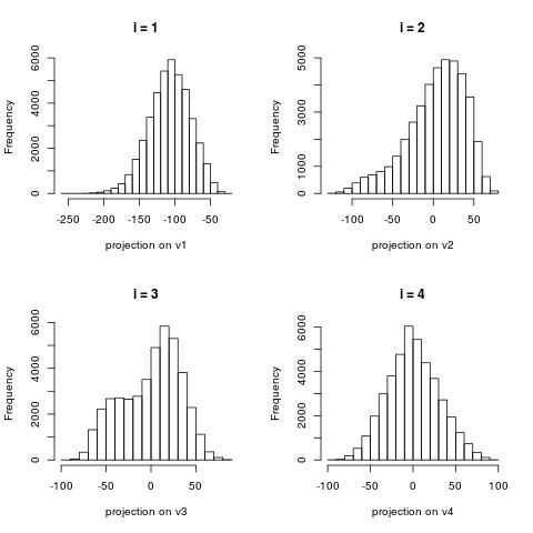
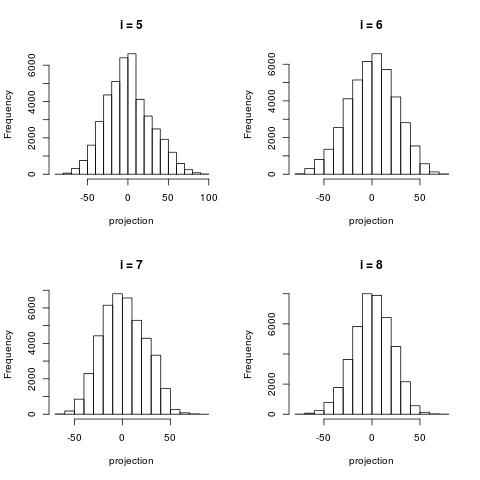
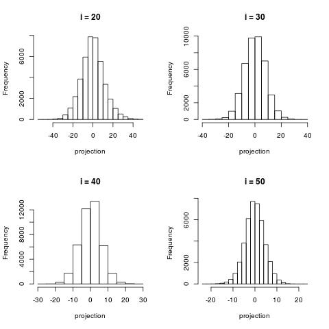
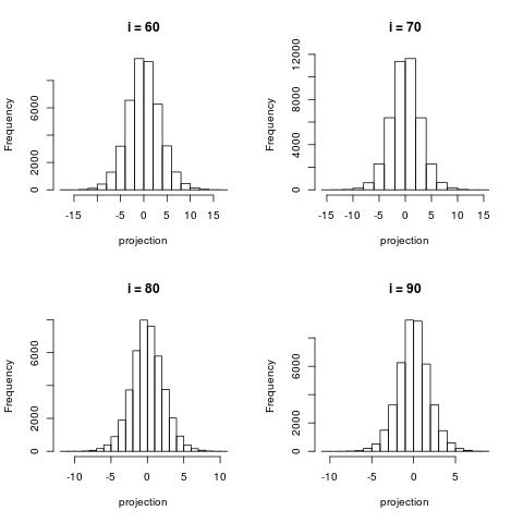
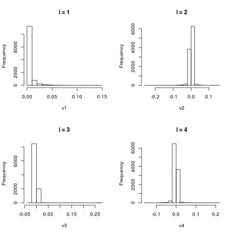
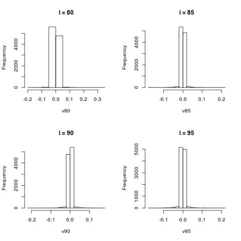
The following histograms are produced by projecting on the $i$-th right singular vector $v_i$. What we can notice is that initially the histograms are non-Gaussian. As $i$ increases, the histograms become progressively more Gaussian (see for example $i = 90$). Another observation is the range of the historam. For $i = 1$, the range is from -250 to 50, then for $i = 2$ the range is from -100 to 50. For large $i = 90$, the range is from -10 to 10. This means that while the contribution of the first singular components is on the order of 50-100, the contribution to the last compoenents is on the order of 10, i.e. 10 times smaller.
The 20 newsgroups dataset consists of roughly 18000 documents on 20 topics. Some of those topics are about politics, sports, regigion and computers. Two particular characteristic of this dataset is that 1) it is a bit noisy (lots of typos and nonsense words) and 2) it is very sparse. If one tokenizes the text (by removing stop words and punctuation, but not stemming), there are more than 100000 tokens. This means that for the task of document classification for which this dataset is typically used there are more “features” in this dataset than data points. Applying the SVD on all the documents and all the tokens may work, but is not great sbecause the dataset is too sparse: many words occur only a few times.
For the purpose of illustration, I restricted the vocabulary about 10000 words by selecting words that appear in at least 10 documents. Then I apply the SVD to find a new (dense) representation of the documents.
What are the conclusions?
First, we want to look at the histograms of the vectors $U[:,i]$ ($i \in 1 \to 100$). These are histograms of the projections of the documents on the vectors $V[:,i]$. We want to see if those distributions look Gaussian and how spread they are. The vectors $V[:,i]$ are “patterns” that SVD extracts. In this case a single “pattern” consists of pairs of (word,score) of all words in the vocabulary. However, the scores for most words close to zero. We’ll see a histogram to verify this. Those “patterns” (may) make sense only when restricting the words with highest scores in absolute values. When we make this restriction we have to look at two cases: words with very high positive scores or words with very high negative scores. Sometimes only one of the groups is present. We’ll see examples.
(A word of warning about Python: I worked with Python’s scipy library for this dataset. However, scipy sparse svd code returns the most significant singular vectors as components with highest indexes, while in Mathematics and other software like R, the most significant singular vectors are returned as components with lowest indexes).
The source code for this example is located here.
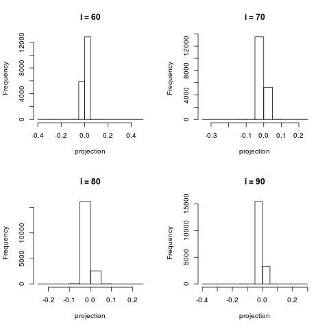
Similarly to the image dataset example, the first right singular vector (the histogram of $U[:,0]$) is about capturing global structure. This vector contains positive components only.
For larger $i$, the histograms become more centered around zero.
For very large $i$, the projection contain very little information and most project are projected close to 0.
Notice that patterns (components) with smaller index $k$ tend to have entries with large absolute values.
The first “pattern” (i = 0) is about capturing the global frequencies of the words. Since some stop words were removed at preprocessing, this list does not contain “the” and “a” but still contains words that are candidates for stop words such as “don” and “does”
i = 0 like 0.147775302271 know 0.147482194479 just 0.146788554272 don 0.146465028471 people 0.126025413091 does 0.122249757474 think 0.121976460054 use 0.108304441177 time 0.104834233213 good 0.104812191112 ... gizwt 5.17132241199e-05 1fp 5.26914147421e-05 u3l 5.5068953422e-05 ei0l 5.64718952284e-05 yf9 5.93467229383e-05 f9f9 5.95880983484e-05 9l3 6.14031956612e-05 nriz 6.14129734355e-05 2tg 6.39805823605e-05 6ei4 6.69369358488e-05
For $i = 1$, the discovered “pattern” reflects one of the topics in the collection: computer related comments (therefore the words “hi” and “thanks” in addition to “windows”, “dos”, “card”). Since this pattern is a line with two directions, one part reflects one topic (computers) while the other end of the line reflects a topic about religion (keywords “jesus”, “believe”).
i = 1 thanks -0.256366501138 windows -0.214518906958 card -0.144940749537 mail -0.118044349449 dos -0.115852183084 drive -0.115360843969 advance -0.112841018523 hi -0.104339793934 file -0.100199344851 pc -0.0985762863776 ... people 0.153422402736 god 0.137434208563 think 0.100187456627 say 0.0897504509532 believe 0.0768755830743 jesus 0.0748355377304 did 0.0737025820581 don 0.0736978005491 said 0.0667736889642 government 0.0589414436946
One more example with $i = 2$.
i = 2 god -0.0276438575267 point -0.0140745932651 drive -0.013190207639 use -0.0128210675667 windows -0.0128185746822 jesus -0.0124390276988 people -0.0122060643629 christian -0.0118160278052 government -0.0116814430183 used -0.0115385485703 ... geb 0.272433495745 dsl 0.269745119918 n3jxp 0.269509373802 chastity 0.269509373802 cadre 0.269205084303 shameful 0.268381119635 pitt 0.26810565487 intellect 0.267277311497 skepticism 0.266284647194 surrender 0.262743742096
In SVD, those patterns are not as clear as in clustering because the production of such patterns in not really part of the objective of SVD. Nevertheless the presence of those “weak” patterns is helpful in initalization of methods whose objective is actually pattern discovery. Such methods are NMF (non-negative matrix factorization) and K-means.
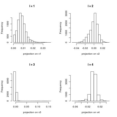
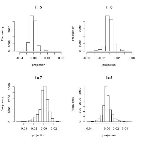
The column vectors $V[:,i]$ represent word patterns as shown in the previous section. Here we just look at the histograms of the scores of those words.
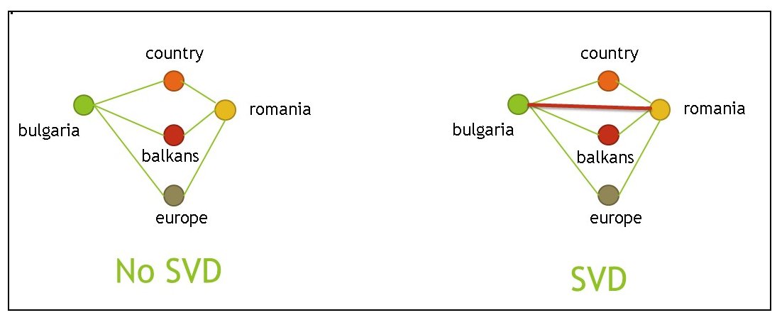
In order to verify that the SVD has been computed correctly I run most similar words queries for a few words. This is mostly for a sanity check. It may not work so well for all words, but should work well for words which are strong topic indicators. The results are below.
neighbors of word windows 0)windows 0.500709023249 1)ms 0.0691616667061 2)microsoft 0.0557547217515 3)nt 0.0533303682273 4)dos 0.0464641006003 5)drivers 0.0365074723089 6)comp 0.0356562676008 7)running 0.0313832542514 8)ini 0.0311252761994 9)application 0.0299640996529 ----------------------------- neighbors of word jesus 0)jesus 0.168165123748 1)christ 0.0782742657812 2)christians 0.0565218749071 3)bible 0.0487185810181 4)christian 0.0407415891892 5)john 0.038291243194 6)sin 0.0368926182977 7)god 0.0343049378987 8)heaven 0.0293666059382 9)jews 0.0282645950168 ----------------------------- neighbors of word congress 0)clinton 0.0236133112056 1)president 0.0161455085553 2)going 0.0160453655028 3)congress 0.0108290114911 4)government 0.0107107140185 5)tax 0.00973937765693 6)bush 0.00902895572165 7)house 0.00886195906841 8)states 0.00885790105693 9)law 0.00824907856166]]>
A lot of Machine Learning textbooks mention the Mahalonobis Distance, but of the textbooks that I have only “The Elements of Statistical Learning” by Hastie, Tibshirani and Friedman mentions the penalized version (which is the version one should use in practice). When I was at univeristy, I was always being warned by my professor: “Never compute the inverse of a matrix unless you have to”. A more useful version of this warning is: “If you want to compute the inverse of the covariance matrix, always smooth the covariance matrix first”.
What is the reason for the professor’s warning? If you analyze the inverse of the covariance matrix though the SVD, you will find out that the inverse entail a division by the covariance matrix singular values (see below). When the input features are correlated you will get some singular values close to 0. So when computing the inverse of the covariance matrix you will divide by a very small number. This will make some of the “newly derived features” very large. This is very bad since those features are the most useless ones for machine learning purposes.
We need some notation to properly describe what happens.
The input data is a matrix $X$ where the rows are the data points and the columns are the features:
X: input matrix rows are data points columns are features.
The (un-centered) covariance matrix is:
If you want the centered version, first compute the mean value for each column and subtract the mean value from its respective column.
Let $X = U S V^T$ be the SVD of $X$.
What we want to accomplish is to compute
$ (X^T X + \lambda I) ^{-1} $
Let $s_1,s_2,\ldots, s_k$ be the first singular values of $X$
Just replace $X$ with its SVD in the formula above. Apply the Woodbery matrix identity and you will work out the answer to be:
$ (X^T X + \lambda I)^{-1} = V \text{diag}\big(\frac{s_i^2}{s_i^2 + \lambda}\big) V^T $
This formula clearly shows
In practical terms, when the number of points is large, but the number of features is small (in the order of 1000’s), we can work with the SVD of the (uncentered) covariance matrix:
where the $V$ and $S$ are the same $V$ and $S$ as in the SVD of $X$. In this way, we don’t require special SVD solvers. You can also use the eigenvalue decomposition since it is the same in this case.
The procedure in this whole blog post can be summarized as:
Step 1. Compute $X^T X$.
Step 2: Compute the svd of step 1: $\text{svd}(X^T X) = V S^2 V^T = V D V^T$. ($D = S^2$)
(Steps 1 and 2 are in case you don’t have a solver for SVD of large matrices. (Check this answer why the svd of $X^TX$ is less desirable to use than the SVD of X)
Step 3: Take the first top $k$ singular values. Those are $d_1 = s^2_1, \ldots, d_k= s^2_k$
Step 4: Compute the transformed features:
Step 5: Compute the Euclidean distance using the transformed features
A little bit of explanation on Step 4 follows. V is a $n$ by $k$ matrix ($n$ is the number of data points). Row $i$ in $V$ is some new representation of the data point. It’s a row vector, let us call it $[v_1, v_2, \ldots, v_k]$. Then we need to put weights to the components of this row vector through $w_i$:
If you want the Mahalanobis Distance first apply the following step 0:
Step 0: Replace each column $col$ in $X$ with $col - mean(col)$. For steps 1 to 5 take $X$ to be the matrix with the replaced columns.
Should you do step 0? It could be that Step 0, makes the solution to Nearest Neighbor worse. Why is that? Typically the features are so encoded that when the value of the feature is close to 0, the feature bears the least information to the problem at hand (for example prediction). So when you subtract the mean, you are making the features less senstive to solving the prediction problem.
]]>That being said, the best use case for the application of the SVD is when the data has multiple weak features (e.g. pixels/words) which are of the same type. Those features should have some structure (correlations) for the SVD to be useful. For example, two neighboring pixels on an image are likely correlated (have similar colors). Ideally features should not have too heavy tailed distribution. This means we don’t want features to take too extreme values too often. This is the reason why for word data we apply some transformations prior to applying the SVD.
Glossary: SVD: Singular Value Decomposition PCA: Principle Component Analysis Mahalanobis Distance: a generalization of Euclidean Distance which takes into account correlation between original features
The formula for the variance of a linear combination of random variables is:
This formula tells us that if two variables are correlated the variance of their sum is increased with twice the amount of their correlation in addition to the sum of the individual variances.
As a simple case consider $\alpha=\beta=1$ and $Var(X) = Var(Y)$. We consider two cases: X and Y are uncorrelated and correlated.
This means that correlation causes the variance of the sum to be twice as large compared to the case when there is no correlation.
A better way to write the above comparision is to create a new feature which is the mean of the two variables:
As it can be seen, averaging uncorrelated variables reduces the variance, while for correlated variables, avaraging did not change the variance (in this case the average is the same variable).
We will consider two use cases for correlation. The first use case is during prediction with linear regression. In this case, when we predict the label of a new data point, we add correlated variables multipled by their estimated coefficients. The coefficients themselves in this case are likely to have high variance. This is why the predicted value will have high variance.
The second use case is related to building stronger predictive features. Strong predictive features tend to have high variance. One way to increase the variance is to add correlated variables to make a stronger feature.
The key difference between those two cases is whether one estimates coefficients based on variables that are correlated or on variables that are not correlated.
Imagine the following situation arising in prediction with linear regression:
There are two sets of variables X1, X2, ..., Xm and Z1, Z2, ..., Zk You want to predict Y as a function of all of those: Y ~ lm(X_i + Z_j) #lm == linear model X1, X2, ..., Xm are correlated. They measure the same signal but with noise: X_i = true X + noise Similarly Z_j's are correlated: Z_i = true Z + noise.
As a practical example $X$ and $Z$ could be two topics. Then $X_i$ are words from the topic $X$ while $Z_j$ could be words from the topic $Z$.
Now I will propose two simple fitting strategies:
Strategy 1: Run linear regression on all the variables: Y ~ lm(X_i + Z_j)
Strategy 2: First average all X_i's and Z_j's: X_mean = mean(X_i) Z_mean = mean(Z_j) Run a regression on X_mean and Z_mean: Y ~ lm(X_mean + Z_mean)
It depends. There are three parameters of importance:
n: number of training points m, k: number of correlated observations (we make m = k for simplicity) noise: how much is the noise due to measurements
However, as we’ll see the first strategy is likely to result in high variance especially in small n and large m and k.
Under the first strategy, let’s imagine we do a stage-wise fitting approach. This means that first we fit to the mean of $Y$, then we choose the better predictor of $X_i$ and $Z_j$. Assume $X_i$ are better predictors. Those variables have essentially the same predictive power, so without loss of generality let us image that we pick $X_1$. At the next state we pick some $Z$, for example $Z_1$. After that none of the remaining variables $X_2$ through $X_m$ and $Z_2$ through $Z_k$ will result in substantial reduction in the error. Their estimated coefficients will be close to 0, but not exactly 0. This is how large variance in the estimated coefficients comes in.
Now there are two ways out:
The second strategy is much better since by averaging, we reduce the variance in $mean(X_i)$ and $mean(Z_j)$. Then we just fit two coefficients which is more stable.
Just want to make clear that L2-penalized regression (or ridge regression) is likely to fix the issue. Internally ridge regression works through the SVD.
In the nearest neighbor prediction model, two data points $a$ and $b$ are similar (or neighbors) if the distance between them is small. As before, let the data points have two components $x_i$ and $z_j$. The variables $x_i$ are correlated between themselves; $z_j$ are also correlated between themselves, but $x_i$ and $z_j$ are not correlated.
Similarly to the regression use case, consider two ways of measuring the distance between $a$ and $b$
Strategy 1: Do not preprocess the variables
Strategy 2: First find the means of x and z, then compute the distance between the means:
Again, why do you want to use the second strategy? Because $x_i$ and $y_i$ are noisy measurements and the distance is not really the “true” distance, but a noisy version with it. The first strategy amplifies the noise present in the measurement, while the second strategy reduces it. The key is to first average the correlated variables to reduce the noise.
A related technique is the so called (penalized) Mahanobis Distance. Mahanonobis distance decorelates the features and normalizes them to have unit variance. Features with very small variances will cause issues unless the penalized version of the Mahalonobis Distance is used. This is where the SVD come in - it makes it possible to better estimate the covariance matrix and to invert it. Be careful with matrix inversion in statistics problems. Always use smoothing techniques. (See the blog post Better Euclidean Distance With the SVD ).
Both euclidean distance and linear regression are expected to work better (lower variance) if the variables are uncorrelated. Therefore the SVD can be motivated by the need to decorrelate the variables.
Now that we know that decorrelation is good, how can we achieve it?
Both the euclidean distance and linear regressioin are based on linear transformation of the original variables. So, it’s natural to consider a reparameterization of the original inputs into new inputs which are linearly related. Assume $x=(x_1,x_2,\ldots,x_m)$ are the original inputs written as a row vector. Then we can consider $k$ new features:
Those features are simply linear combinations of the original features. There are two natural requirements of those features:
The new features $f_j$ are uncorrelated
The new features $f_j$ have high variances
A third (technical) requirement is that the L2-norm of the coefficients $\beta_{j}$ is 1.
The first requirement is motivated by the previous discussion how correlation results in a large variance of the preditions. The second requirement states that $f_j$ should have high variances. Why? Consider what happens under the opposite possibility, namely that $f_i$ have small variances. The smallest variance is zero, which means that the variable is a constant. A constant will yield no information neither for regression nor for computing the closes points with euclidean distance. Large variance of the feature means exactly the opposite. It means an informative (discriminative) feature. For example, making measurements of the feature more fine grained will increase the information (variance/entropy) of the feature in general.
Now one can try the following stagewise approach:
Stage 1: Find the linear combination of the original features that has the highest variance. Stage 2: Find a second linear combination which is uncorrelated with the first, but again with largest possible variance. Stage 3: A linear combination uncorrelated with the first and the second derived feature and maximal variance ...
As it happens, this procedure is equivalent to the PCA. PCA is the SVD not of the original input features, but of the feature minus their respective means. This is because the formula for the covariance requires subtracting the means. For now we’ll keep this intuition, but later on we’ll compare the SVD to the PCA (i.e. in what cases subtacting the means of the orignal variables makes sense).
As it can be seen from the stagewise algorithm, each subsequent feature has less variance (less information). However, the variance of the feature has two components:
Since we systematically exhaust the structure, at the end we are left mostly with noise. The common wisdom is that we just keep the first few linear combination (50 to 500) depending on the size of the data and drop the rest.
It may be that for some data points, the optimal choice is 50 features from the SVD while for other datapoints the optimal is 5 features. We should also be aware that data points with norms close to 0 (such as data points having fewer measurements as well as outliers) will not be well-represented by the SVD. This means the structure behind those data points is not found, but noise is added nonetheless. The noise comes from imposing a structure based on other data points. That’s why this argument about SVD cleaning the noise, while true on average, is wishful thinking for some data points. This will be a separate blog post on that issue with worked example as well as advice what to do about the issue.
It is optimal in the sense of the mathematical model just described: that we can decompose the original features into a smaller number of features while preserving most of the variance (interesting structure) of the dataset. But what are the shortcoming to this approach:
Latent Semantic Indexing was proposed in 1990 by a team of researchers of which Susan Dumais is the most prominent. She is currently a Distinguished Scientist at Micorosft Research. LSI was proposed as a text search technique.
Latent Semantic Analysis was proposed in 2005 by Jerome Bellegarda for natural language processing tasks. Bellegarda showed massive improvements in speech recognition tasks due to the ability of the LSA to capture long-term (or semantic) context of text.
SVD, the underlying technique behind LSI/LSA, is a statistical technique known for a very long time in Statistics and Linear Algebra. In Statistics, SVD is particularly useful in the context of linear regression.
Susain Domain (the original author of LSI) was elected an ACM fellow in 2006 partly because of her LSI contribution, while Jerome Bellegarda was elected an IEEE fellow in 2004 partly due to LSA. These are very high awards speaking to the importance of this method.
You can calculate that currently LSI is 25 years old while LSA is 10 years old. SVD is known for a much longer time.
LSA was highly hyped at the time of its introduction, but it took a bit more time to researchers to properly understand the strengths and weaknesses of the method. No one, as far as I know, could achieve similarly high improvement in perplexity reduction as Bellegarda. However, (Google) word vectors, a similar approach (at least in spirit) to LSA reported high improvement in perplexity reduction.
In the field of Information Retrieval, some textbooks state that no improvement in precision was achieved in search tasks after application of the LSI. However, application of LDA (Latent Dirichlet Allocation) reported improvement in search tasks. LDA was motivated as an improvment of Probabilistic Latent Semantic Analysis (PLSA), which itself was motivated as an improvement of LSA.
Here is a table of ancronyms used in machine learning/data mining literature:
SVD: Singular Value Decomposition. A standard technique from Linear Algebra and Statistics. LSI: Latent Semantic Indexing. An application of SVD in Information Retrieval. LSA: Latent Semantic Analysis. LSI applied to natural language processing. PLSA: Probabilistic Latent Semantic Analysis. An improvement to LSA. LDA: Latent Dirichlet Allocation. An improvement to PLSA. PCA: Principle Component Analysis. A statistical technique which is an application of SVD.
In 2009, SVD became popluar in recommendation systems due to the Netflix Prize competition. It was one the few stand-alone methods that achieved good results. One difference from prior work is the so called the smoothing trick of adding a small diagonal matrix before taking the SVD. This trick was not mentioned neither in the LSI or LSA work (however it is well-known in statistics in the context of ridge regression and penalized PCA). So tricks are important and part of this blog post series is about the tricks that I have learned along the way.
I plan to deconstruct the LSA (LSI, SVD) in order to separate fact from fiction and show some practical tricks. I also plan to show that SVD does not work well for some data points (words or documents) when applied to text.
One should keep in mind that even though LSI/LSA/SVD is an old method, the principles behind the method are still valid. Follow up work on Latent Dirichlet Allocation has improved search, and (Google) Word Vectors have improved the NLP perplexity reduction tasks.
Meanwhile, big data requirements motivated the development of fast algorithms for computing cheaply the SVD of a huge matrix (those aglorithms are randomzied). At the same time, SVD has been accepted in the industry. Some companies are applying the SVD (or related techniques such as LDA) in their recommendation systems.
]]>Here is the recipe:
Input: dataset (n by m matrix where n datapoints(rows) m features(columns)) Step 1: Apply svd to the original dataset decor_dataset = svd(dataset) # decorrelated dataset this is an n by k matrix, k dimensions after reduction) Step 2: Build randomized trees for i until num trees do random_matrix = generate a hadamard matrix of dimension k by s do not choose s to be more than 4*log(n) because it's not necessary and you'll save computation randomized_dataset = decor_dataset %*% random_matrix at each tree node simply choose a single feature (the features are orthogonal to each other) Step 3: Run nearest neighbor for each point in the dataset and store the top 10 neighbors in the index
On very sparse data random projections will not perform well. This is known. So it is better to make the data denser. Use SVD for this. (One can apply random projections on the sparse data to make it dense. However, it is known that random projections will need more dimensions than the SVD. Fewer dimensions will make the search easier. That’s why I recommend the SVD.)
Even when the data is dense, it is recommended to apply the SVD. Why is that? Because the efficiency of random projections drops when it has to deal with correlated features.
It is known how to make the SVD fast and scalable and even how to make it work as an online algorithm, so SVD is not really a bottleneck.
There are many ways to build randomized trees. But after some experimentation the following properties emerged:
If you build trees with standard random projections, then a computation at a non-leaf node (to choose whether to go to the left or right child) will take time proportional to the number of features (e.g. 100). This is simply too much when just splitting on one single feature will suffice. So, it is essential to have run the SVD to sphere the data. The multiplication of the data by a random matrix before building the tree is simply a random rotation of the dataset. This is necessary to guarantee that different trees will explore the space of the points in different ways.
On point 2. What are good trees? It means that if two points are really nearest neighbors, then they should end-up together (in the same leaf) in many trees. For high-dimensional and very noisy data, this might not happen.
Point 2 simply means: if we explore the space in two different (random ways), we should end-up at the same conclusion “sufficiently” often.
This matrix is a special matrix whose columns are orthogonal. Simply, it is a number of random projection column vectors stacked next to each other. However, this matrix has a special structure that allows a computation of a vector of size $k$ by this matrix (which itself has size k x k) to take $k \times log(k)$ steps and not $k \times k$ steps. This is a huge saving.
You don’t need to generate the Hadamard matrix to multiply by it. Use the following recursive algorithm.
Multiply by Hadamard input: a vector of numbers multiply the input by random numbers (gaussian or bernoulli) call loop(input) output: the same vector under random rotation def loop(input): (a,b) = split(input) # split at length(input)/2 result_a = loop(a) result_b = loop(b) if length(a) == length(b): # case 1 create a vector by appending one after each other return append( (result_a + result_b), (result_a - result_b)) else # case 2 # one vector is bigger (assume it's the vector a) # it must be bigger by one position only let result_a' = result_a[0:length(result_a) - 1] let last_a = result[length(result_a) - 1] result_a' and result_b are of the same length. handle like case 1 let rand_b = result_b[random_pos] let random_sign = +1 or -1 return append( (result_a' + result_b), [last_a + random_sign*rand_b], (result_a' - result_b) )
Nearest neighbor search is an approximate algorithm. In order to improve it the following heuristic might be useful:
The neighbor of a neighbor is likely a neighbor.
At query time do the following:
Query time: - compute the approximate neighbors using the index (from steps 1 and 2) - get the neighbors of the neighbors (that's why we need them precomputed) - some of those might be a better neighbor because of the approximation
There is actually a method for nearest neighbor search called K-graph that works entirely on this principle.
]]>This series contains tips and tricks about the SVD. SVD is a foundational technique in Machine Learning. This series approaches the SVD from a few view points to build more useful intuition what is actually happening behind the equations.
The equation behind SVD is a very elegant mathematical statement, but also a very “thick” one as well.
The SVD of a matrix is defined as
In data problems, $X$ is typically the dataset, and the SVD helps create a more “condensed” representation. Although a simple statement to state, it is not so simple to understand what this statement gives us.
As a data scientist, I prefer much more the following way to write the SVD:
This way to write the SVD gives as the interpetation that SVD extract patterns from the data represented by columns of the matrix V. This is the red and green column in the picture. Then each data point is compared with the patterns via the dot product. The dot product is a way to measure overlap. In the end, the matrix U gives us a new representation of the data based on the patterns discovered in the original dataset.
SVD is used in Search, Recommendation Systems and Natural Language Processing. In those fields the application of SVD is known under the names of Latent Semantic Indexing or Latent Semantic Analysis.
Check out the sidebar for more topics.
]]>