SVD: The Projections View
2D Geometry
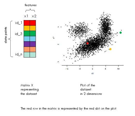
When the dataset has two features, one can visualize the whole dataset on a 2D plot.
Let the data be represented by the matrix $X$ where rows are data points and columns are features.
Projection of a single point
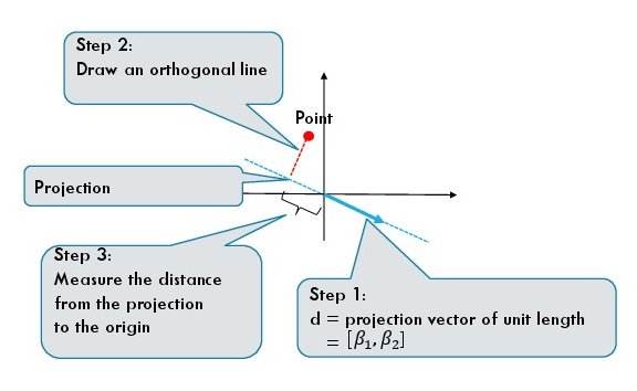
For a one dimensional projection we require a direction which is given by a unit vector $d = [\beta_1, \beta_2]$. The projection of each data point is given by the dot product of the feature vector and the direction:
The above equations give us a procedure to geometrically find the projection of a data point.
- First, we draw a directed line given by the vector $d$.
- Second, we find the point on the projection line which is closest to the data point. The closest point is the projection of the original data point.
- We measure the directed distance (it can be negative) from 0 to the projected data point.
Projection of a dataset
The projection of a single point is not informative unless we compare it with the projection of all other points.
Projecting the whole dataset in one dimension gives us a histogram. This histogram is somewhat informative because it may reveal some structure from the original dataset.
Here is an example. This dataset has two clusters.
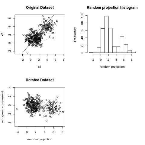
We can observe the clustering structure in the projection above. However, we cannot observe the clustering structure on the projection below.
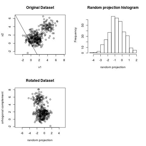
The projection of largest variance does not necessarily reveal the clustering structure.
It is known that PCA (a technique related to SVD) is related to finding projections where the histograms are as wide as possible (a wide histogram means large variance). The projection of largest variance is the widest histogram. However, the largest variance projection does not necessarily capture the clustering structure or separability between clusters. This is somewhat of a textbook statement since many textbooks mention this fact.
In the example below we have two clusters which are separable across the axis $x_2$. The dominant right singular vector is however along the direction $x_1$. The singular values are 15 and 6 which tell us that the variance along $x_1$ is about 2.5 times larger than the variance along $x_2$. The clustering structure is revealed however by the second right singular vector of the SVD which is along $x_2$.
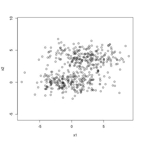
An example where no one dimensional projection can capture clustering structure
It is an interesting question whether for a given dataset we can find one dimensional projections from which you can read the clustering structure (i.e. the histogram of the projection has two peaks and you can guess the clusters from the histogram). This is not possible.
Here is an example with three spheres at equal distance from each other. When projected in one dimension we are never going to see the clusters clearly.
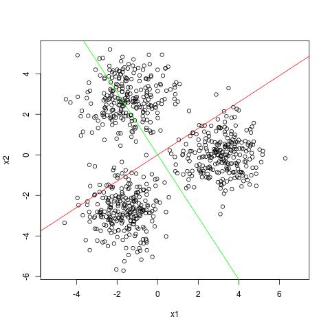
The red and green line are the first and second dominant singular vectors.
However, SVD is still useful for finding clusters in the dataset (see my blog post on SVD and clustering [TO APPEAR]).
Interesting stuff is in the corners of the projection
Imagine that the data lies on a unit sphere. This is the case when the cosine similarity is used. As it can be seen from the figure below points which are projected in the corners of the projection line are likely to be situated in a much smaller region than points which are projected in the middle. One can have two points projected in the middle which are diametrally opposite each other. In the figure, those are some of the yellow points.
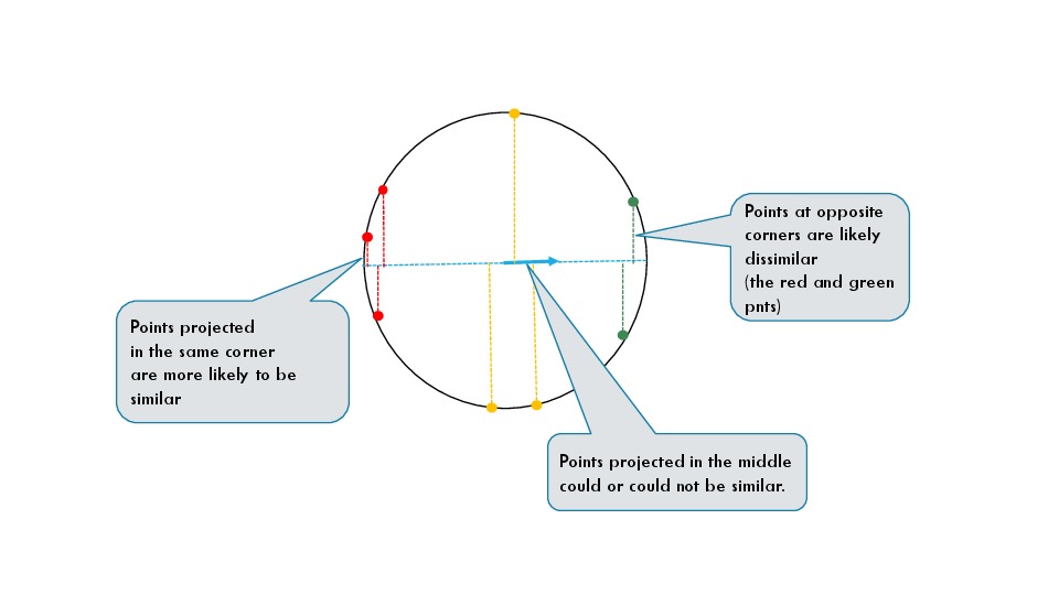
The value of thie statement is that if you take some points projected in one of the corners, those points are likely highly similar. On the other hand, SVD will choose projections for which more data is projected in the corners. This means that the SVD extracts some dominant patterns from the data.
The last statement is used as a heuristic for initialilization of the K-Means clustering algorithm. In the three cluster example above (titled: no one dimensional projection can capture clustering structure), one can see that three of the four corners of the projections contain points from distinct clusters. Points from different corners could be useful for initial centroids in K-means.
High-Dimensional Geometry
Some of the intuition about one dimensional projections carries over to high dimensions. In particular, a one dimensional projection (the histogram) is a view of the dataset also in high dimension. However, it is a much noiser view than a projection in 2D.
In high dimensions it is much more likely that most of the dataset ends up in the middle of the histogram. Why is that? Think of the case of documents on the web. What is a projection is this case? It is two sets of words each representing a topic (why two sets? because the line on which we project has two directions). As an example of two sets of words consider sports and politics. Now projecting a point means that we compare a document on the spectrum from sports and politics. Most documents will be about neither of those things. So those documents (datapoints) are projected close to 0. Projection is dot product and dot product is overlap. A random document will have no overlap with sports or politics. So, in high-dimensions for most possible projections, most of the dataset is projected in the middle. (There is a formal mathematical theorem about this phenomenon.)
The intuition from 2D about the corners of the projections carries over. This means that we should seek interesting structure in the corners. However, there are too many corners in high dimensions and too little data projected on those corners.
SVD/PCA is about seeking interesting projections
The following is the common notation:
The SVD of $X$ is given by
We can write this equation as
This is possible because $V V^T = I$ ($V$ is an orthonormal matrix).
Let us take $V$ to have only one column (this is the truncated SVD with $k = 1$), i.e.$V$ is a single column vector of dimension $m$. This is a projection direction as we described above. Now $U$ is a single column vector $u$ as well, however of dimension $n$. In this case $S$ is a single number $s_1$. $u$ contains the coordinates of the projected points.
We know the following is the best rank-1 approximation to the matrix $X$:
Therefore, we can argue that the projection on the first component of the SVD is the projection that will in some sense “best preserve” the dataset in one dimension. Typically this first projection of the SVD will capture “global structure”.
One way heuristic way to think about the first component is as follows. Think of $v_i$ as the average of the $i$-th column; think of $u_j$ as the average of the $j$-th row. This procedure is (sometimes) a heuristic approximation to the SVD with one dominant component when the dataset has global structure. You can see that this is confirmed in the MNIST dataset example below.
PCA projections
One way to define “interesting” is away from normal. One way to be away from normal is to have high variance (heavier tails). The PCA takes exactly this route. It finds the projections which have the highest variance. One critical difference from the SVD is that PCA is SVD on the data after subtracting the means.
Example with MNIST (Image data)
Here we want to see how the projections that the SVD produces look like. The MNIST dataset consists of 42000 images. Each image is represented as a 784 dimensional vector. One can obtain this digit recognizer dataset from Kaggle.
I use the following code to read the data and compute the matrix V
train_data <- read.csv('../data/train.flann', header = FALSE, sep = " ")
X <- sqrt(data.matrix(train_data))

num_examples <- dim(X)[1] #n
num_features <- dim(X)[2] #m

#The sample covariance matrix
XtX <- (t(X) %*% X)/(num_examples - 1)
s <- svd(XtX)
The projections are computed with the following code:
k = 100 #number of singular vectors wanted
V = s$v[, 1:k]

lam <- 50
d <- s$d[1:k]
weights <- sqrt(d/(d + lam))

Vweighted <- s$v[, 1:k] %*% diag(weights)


projections = X %*% Vweighted
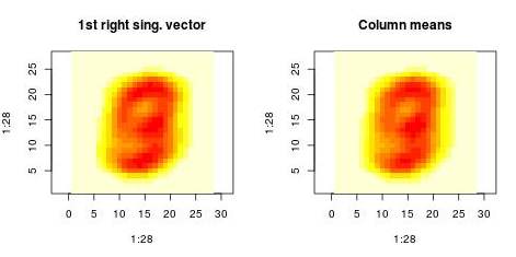
First, I want to make sense of the first projection. We compare the projection on the first right singular vector (on left plot) and the projection on the centroid of the dataset (right plot). Those histograms are very similar and the correlation coefficient beween both projectons is 0.999
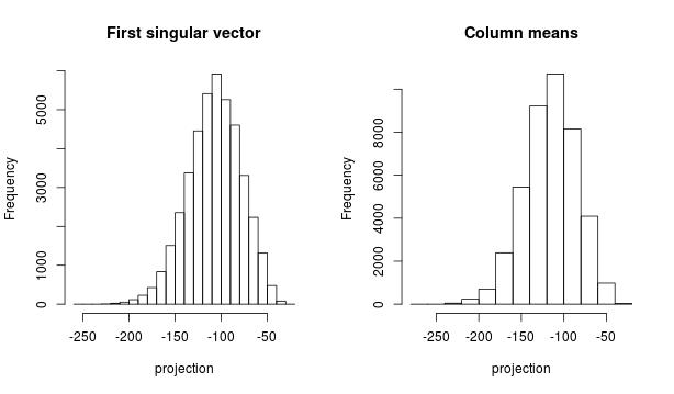
This is the code I used to compute the histograms above.
X_colMeans = -colMeans(X)
#projection on the column means
proj_colMeans = X %*% matrix(X_colMeans, byrow = FALSE)

hist(projections[,1], xlab = "projection", main = "First singular vector")

#divistion by norm of col means to put the data on the same scale as projections[,1]
norm_colMeans = sqrt(sum(X_colMeans * X_colMeans)) #107.6
hist(proj_colMeans/norm_colMeans, xlab = "projection", main = "Column means")

cor(projections[,1], proj_colMeans)
This means that the SVD first finds the global structure by “averaging” all images. Then it subtracts this structure and contininues recursively to find additional structure.
We can also examine the “patterns” present in the right singular vector ($v_1$) and in the
vector constructed by averaging columns:
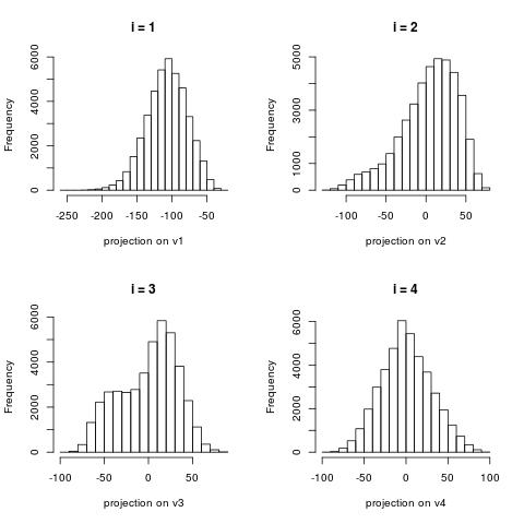
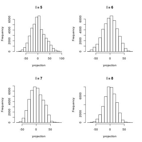
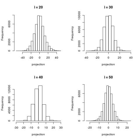
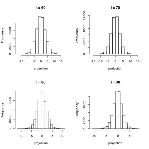
The following histograms are produced by projecting on the $i$-th right singular vector $v_i$. What we can notice is that initially the histograms are non-Gaussian. As $i$ increases, the histograms become progressively more Gaussian (see for example $i = 90$). Another observation is the range of the historam. For $i = 1$, the range is from -250 to 50, then for $i = 2$ the range is from -100 to 50. For large $i = 90$, the range is from -10 to 10. This means that while the contribution of the first singular components is on the order of 50-100, the contribution to the last compoenents is on the order of 10, i.e. 10 times smaller.
Example with 20 Newsgroups (Text data)
The 20 newsgroups dataset consists of roughly 18000 documents on 20 topics. Some of those topics are about politics, sports, regigion and computers. Two particular characteristic of this dataset is that 1) it is a bit noisy (lots of typos and nonsense words) and 2) it is very sparse. If one tokenizes the text (by removing stop words and punctuation, but not stemming), there are more than 100000 tokens. This means that for the task of document classification for which this dataset is typically used there are more “features” in this dataset than data points. Applying the SVD on all the documents and all the tokens may work, but is not great sbecause the dataset is too sparse: many words occur only a few times.
For the purpose of illustration, I restricted the vocabulary about 10000 words by selecting words that appear in at least 10 documents. Then I apply the SVD to find a new (dense) representation of the documents.
What are the conclusions?
First, we want to look at the histograms of the vectors $U[:,i]$ ($i \in 1 \to 100$). These are histograms of the projections of the documents on the vectors $V[:,i]$. We want to see if those distributions look Gaussian and how spread they are. The vectors $V[:,i]$ are “patterns” that SVD extracts. In this case a single “pattern” consists of pairs of (word,score) of all words in the vocabulary. However, the scores for most words close to zero. We’ll see a histogram to verify this. Those “patterns” (may) make sense only when restricting the words with highest scores in absolute values. When we make this restriction we have to look at two cases: words with very high positive scores or words with very high negative scores. Sometimes only one of the groups is present. We’ll see examples.
(A word of warning about Python: I worked with Python’s scipy library for this dataset. However, scipy sparse svd code returns the most significant singular vectors as components with highest indexes, while in Mathematics and other software like R, the most significant singular vectors are returned as components with lowest indexes).
The source code for this example is located here.
Histogram of documents projected onto the right singular vectors (i.e. histograms of the column vectors $U[:,i]$)
Similarly to the image dataset example, the first right singular vector (the histogram of $U[:,0]$) is about capturing global structure. This vector contains positive components only.
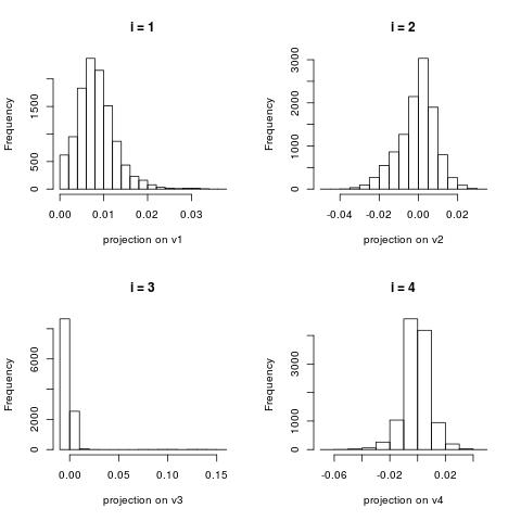
For larger $i$, the histograms become more centered around zero.
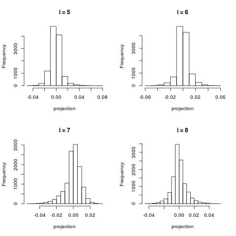
For very large $i$, the projection contain very little information and most project are projected close to 0.
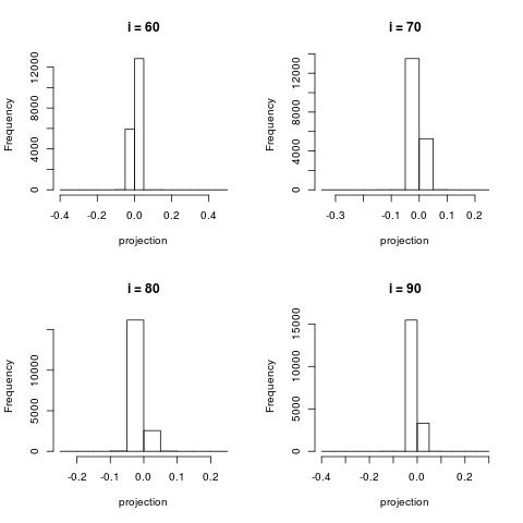
Some patterns (those are the vectors $V[:k]$)
Notice that patterns (components) with smaller index $k$ tend to have entries with large absolute values.
The first “pattern” (i = 0) is about capturing the global frequencies of the words. Since some stop words were removed at preprocessing, this list does not contain “the” and “a” but still contains words that are candidates for stop words such as “don” and “does”
i = 0

like	0.147775302271
know	0.147482194479
just	0.146788554272
don	0.146465028471
people	0.126025413091
does	0.122249757474
think	0.121976460054
use	0.108304441177
time	0.104834233213
good	0.104812191112
...
gizwt	5.17132241199e-05
1fp	5.26914147421e-05
u3l	5.5068953422e-05
ei0l	5.64718952284e-05
yf9	5.93467229383e-05
f9f9	5.95880983484e-05
9l3	6.14031956612e-05
nriz	6.14129734355e-05
2tg	6.39805823605e-05
6ei4	6.69369358488e-05
For $i = 1$, the discovered “pattern” reflects one of the topics in the collection: computer related comments (therefore the words “hi” and “thanks” in addition to “windows”, “dos”, “card”). Since this pattern is a line with two directions, one part reflects one topic (computers) while the other end of the line reflects a topic about religion (keywords “jesus”, “believe”).
i = 1

thanks	-0.256366501138
windows	-0.214518906958
card	-0.144940749537
mail	-0.118044349449
dos	-0.115852183084
drive	-0.115360843969
advance	-0.112841018523
hi	-0.104339793934
file	-0.100199344851
pc	-0.0985762863776
...
people	0.153422402736
god	0.137434208563
think	0.100187456627
say	0.0897504509532
believe	0.0768755830743
jesus	0.0748355377304
did	0.0737025820581
don	0.0736978005491
said	0.0667736889642
government	0.0589414436946
One more example with $i = 2$.
i = 2

god	-0.0276438575267
point	-0.0140745932651
drive	-0.013190207639
use	-0.0128210675667
windows	-0.0128185746822
jesus	-0.0124390276988
people	-0.0122060643629
christian	-0.0118160278052
government	-0.0116814430183
used	-0.0115385485703
...
geb	0.272433495745
dsl	0.269745119918
n3jxp	0.269509373802
chastity	0.269509373802
cadre	0.269205084303
shameful	0.268381119635
pitt	0.26810565487
intellect	0.267277311497
skepticism	0.266284647194
surrender	0.262743742096
In SVD, those patterns are not as clear as in clustering because the production of such patterns in not really part of the objective of SVD. Nevertheless the presence of those “weak” patterns is helpful in initalization of methods whose objective is actually pattern discovery. Such methods are NMF (non-negative matrix factorization) and K-means.
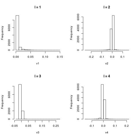
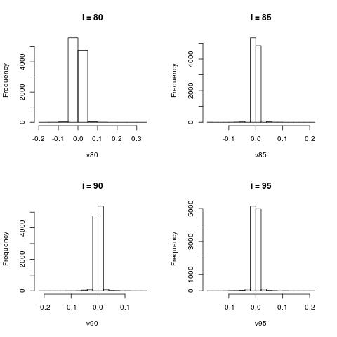
Histograms of $V[:,i]$
The column vectors $V[:,i]$ represent word patterns as shown in the previous section. Here we just look at the histograms of the scores of those words.
Finding similar words after application of the SVD
In order to verify that the SVD has been computed correctly I run most similar words queries for a few words. This is mostly for a sanity check. It may not work so well for all words, but should work well for words which are strong topic indicators. The results are below.
neighbors of word windows
0)windows	0.500709023249
1)ms	0.0691616667061
2)microsoft	0.0557547217515
3)nt	0.0533303682273
4)dos	0.0464641006003
5)drivers	0.0365074723089
6)comp	0.0356562676008
7)running	0.0313832542514
8)ini	0.0311252761994
9)application	0.0299640996529

-----------------------------
neighbors of word jesus
0)jesus	0.168165123748
1)christ	0.0782742657812
2)christians	0.0565218749071
3)bible	0.0487185810181
4)christian	0.0407415891892
5)john	0.038291243194
6)sin	0.0368926182977
7)god	0.0343049378987
8)heaven	0.0293666059382
9)jews	0.0282645950168

-----------------------------
neighbors of word congress
0)clinton	0.0236133112056
1)president	0.0161455085553
2)going	0.0160453655028
3)congress	0.0108290114911
4)government	0.0107107140185
5)tax	0.00973937765693
6)bush	0.00902895572165
7)house	0.00886195906841
8)states	0.00885790105693
9)law	0.00824907856166