Beyond Cosine Similarity
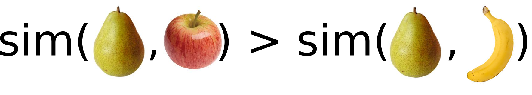
Most people would agree that pears are more similar to apples than to bananas.
However, it comes to the algorithmic comparison between documents, pronouncing documents as similar using computer code is not that straightforward. I personally feel that more powerful and precise concepts should be used than just to talk about “similar” documents.
For one thing, the widely used cosine similarity is the worst performing one in a recent study. Recent experimental results by Computer Science Professor Charles L.A. Clarke and John S. Whissell in their paper “Effective Measures for inter-document similarity” show that statistically founded methods perform much better than similarity based on cosine.
For the purpose of this post, I understand similarity as defined in Wikipedia: the inverse of a distance.
Typical uses of document similarity
Document similarity is typically used in the following areas:
- Ranking in Information Retrieval
- Document classification
- Document clustering
Beyond Cosine: A Statistical Test.
Instead of talking about whether two documents are similar, I would prefer to talk whether two documents come from the same distribution. This is a much more precise statement since it requires us to define the distribution which could give origin to those two documents. More over, using the machinery of statistical tests we have proper procedures for deciding whether two documents are similar. The kind of test applicable to test similarity is known in the statistics literature as a test of homogeneity.
Often similarity is used where more precise and powerful methods will do a better job. The following are some warning signs when similarity is being used suboptimally:
- Using a symmetric formula, when the problem does not require symmetry. If we denote sim(A,B) as the similarity formula used, the formula is symmetric when sim(A,B) = sim(B,A). For example, ranking documents based on a query, does not work well with a symmetric formula. The best working methods like BM25 and DFR are not similarities in spite of the term used in the Lucene documentation since they are not symmetric with respect to the document and query. As a consequence of the preceding point similarity is not optimal for ranking documents based on queries
- Using a similarity formula without understanding its origin and statistical properties. For example, the cosine similarity is closely related to the normal distribution, but the data on which it is applied is not from a normal distribution. In particular, the squared length normalization is suspicious.
Deriving similarity from a hypothesis test
If we adopt the standard bag of words model, a document is represented as a set of counts or equivalently a document is a multinomial probability distribution over words. To make the result presented below more concrete I start with some basic definitions.
Two documents (document 1 and document 2) are represented as normalized counts, or multinomial probability distributions.
- $P = (p_1, p_2, p_3, …, p_N)$ is the multinomial distribution of the words in document 1. $p_{i}$ = count(word(i))/length(document 1)
- $Q = (q_1, q_2, …, q_N)$ is the multinomial distribution of the words in document 2. $q_{i}$ = count(word(i))/length(document 2)
- N = total number of words in English (or collection)
Using the terminology from statistical hypothesis testing, let H_0 and H_alt denote the null and the alternative hypothesis respectively.
The statistical test is:
- $H_0$: $p_{1} = q_1$ and $p_2 = q_2$ and … and $p_N = q_N$
- $H_1$: the opposite of $H_0$, i.e. at least for one $i$: $p_i \neq q_1$
Solving the above formulation leads to the use of the Jenson-Shannon divergence as a test statistic or document similarity. The Jensen-Shannon divergence is closely related to the Kullback–Leibler divergence (KL distance). The KL distance can be approximated by the Chi-Square Test Statistic with which more people are familiar.
For one possible derivation of the Jenson-Shannon divergence as a test statistic one can consult formulas 52 to 57 in http://research.microsoft.com/en-us/um/people/minka/papers/minka-multinomial.pdf
Here is the resulting test statistic or similarity between two documents with distributions P and Q:
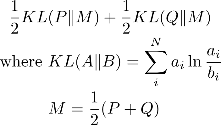
KL(A||B) can be interpreted as an “asymmetric distance” between distributions A and B. M is the average between the distributions P and Q. Based on the above formula, Jensen-Shannon divergence has the procedural interpretation:
We create the average document M between the two documents 1 and 2 by averaging their probability distributions or merging the contents of both documents. We measure how much each of the documents 1 and 2 is different from the average document M through KL(P||M) and KL(Q||M) Finally we average the differences from point 2. Potential issue: we might want to use weighted average to account for the documents lengths of both documents.
The Jenson-Shannon divergence can also be written as follows:

The interpretation of the above is as follows: We create the average (merged, mean) document $M = \frac{1}{2}(P + Q)$ and we compress it. The LogLik is the negative of the compressed document length. We compress each of the documents 1 and 2 individually and we add their compressed lengths. -LogLik(P) and -LogLik(Q) are the lengths of the compressed documents 1 and 2. We compare the results from point 1 and point 2. If both documents were to come from the same distribution, the average document will actually compress much better than if we had compressed documents individually. This is so, because the merged (mean) document M will exploit the redundancy (commonality in representation) in individual documents.
Mathematical Derivation
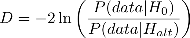
It is helpful to derive the Jenson-Shannon formula from the hypothesis test itself. The machinery of hypothesis testing involves the so called likelihood ratio test and the related Neyman–Pearson lemma which justifies its usage.
The first step is to form the difference test statistic D:
| P(data | H_0) is the probability that we see the observed data, or in our concrete case the document word counts, given that the null hypothesis were true. |
If the null hypothesis were true, then we observe two independent samples, the counts of document 1 and the counts of document 2. Given two independent samples, how does one estimate the unknown probability distribution, which is most likely to have generated the documents. Here we switch from hypothesis testing to estimation. We have to find out what good estimation methods are there for multinomial distributions. From the literature of Information Retrieval we know that the preferred methods involve the so called smoothing technique. One standard reference to consult on this topic is “A study of smoothing techniques on language models” by Lafferty and Zhai). The probability of the data given H_0 is given by:
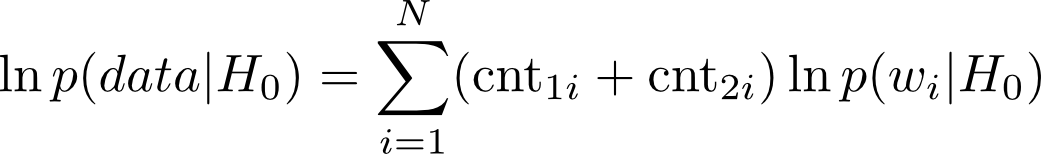
In the above cnt_{1i} and cnt_{2i} are the counts of $word_i$ in documents 1 and 2 respectively.
The key to successful usage of the above formula is to use a good technique of estimating the probability of a word under $H_0$ P(w_i|H_0). The standard choice is to use Dirichlet smoothing as specified in the Lafferty and Zhai paper. I am not going to dwell on this issue, but will only say that using a proper smoothing method makes a difference between the formula not working and working well. The use of smoothing has two interpretations:
First, it empowers the model with knowledge of English via the frequencies of words in English Second, it turns out that the usage of frequencies in English in smoothing results in downplaying the contributions of stop words.
Conclusion
In this blogpost, I showed an honest and rigorous derivation of one statistical method for measuring the similarity between two documents. I called the derivation honest in the sense that in every step of the way I was listing the assumptions I make. The cosine similarity is not really honest since its assumptions are not clearly stated. More over, by being explicit about the assumptions, we can actually consider if they hold for our data and we can test them. We can also revisit and modify some assumptions. For example, we could include assumptions about document length, change the multinomial distribution to a Poisson distribution and even include expansion through related words. The test of homogeneity hypothesis test method is general as it allows us to use the same framework and adapt even BM25 and DFR formulas from text search to “symmetric” document similarity.
Recommended Additional Reading
- “Semantic Smoothing of Document Models for Agglomerative Clustering” by Xiaohua Zhou, Xiaodan Zhang, Xiaohua Hu. This paper shows application of smoothed symmetrized KL-distance to hierarchical agglomerative clustering of documents.
- Blog post “KL-divergence of two documents” by Manos Tsagkias. Describes another version of symmetrized KL-divergence, smoothing and includes some Python code.
- “Bayesian inference, entropy, and the multinomial distribution” by Thomas Minka from Microsoft Research. It shows derivation of Jenson-Shannon divergence in the context of Hypothesis testinig framework.
- “Using Kullback-Leibler Distance for Text Categorization” by Brigitte Bigi. Describes the usage of symmetrized KL-divergence (called KL-distance) to text categorization task. Includes comparison to cosine similarity.